Volatility term structure from multiple angles (part 1)

The post Dragonfly Eyes served as a broad preamble to our exploration today. Be like a dragonfly — look through multiple lens.

We’re going to expand our thinking about volatility term structure to see why it’s a diamond with several facets — and most interestingly — why multiple ways of looking at it are not all correlated.

We are going to consider volatility term structure in a few ways. The differences will make the value of multiple lenses self-evident. The source of the differences have highly practical ramifications for 3 tasks:

1. risk management
2. surface modeling
3. trade prospecting

I would be surprised if even an experienced trader didn’t walk away folding the Rubik’s cube known as vol term structure in their head. If anything, I’m sure a seasoned trader can find some interview questions embedded in the concepts to bounce off candidates.

If you are a novice trader, you will still benefit. There’s nothing more than arithmetic in here. The value of hacking ideas from several vantage points will be obvious plus you will learn some basic transformation and measures that the more experienced folk take for granted.

About this post

• The post is the first of a 2-parter. It won’t all fit in the single email view plus I’ve been under the weather this week. All the background work is done but I’m running on fumes to write it all up.
• It’s a semi-Socratic progression of “show don’t tell” which serves to make the lessons your own.
• We will use GLD vol data for the past year which was whimsically chosen. I didn’t snoop at the data first.
• We get into implications for your own procedures.*
• Finally, I talk about how and why I will extend the analysis.

*The word “your” prompts a reasonable question — who’s this for? I’m imagining a trader or risk manager at a prop shop/asset manager or an extremely sophisticated retail option trader. The material comes from pragmatism and experimentation. A durable way of seeing based on lots of pain. This is the stuff of salt mines. The way traders think.

Where does this intersect with quant and formal risk management?

Everywhere.

Quants may have a different language and set of methods for computation but the concerns are the same. I’ve said it before, but the caricature of the ivory tower theoretical physics PhD without street smarts is foreign to me. All of the gigabrain quants I’ve worked with were both practical and exceptional at asking questions. Their priority was reality.

Their knowledge becomes indispensable as risk management scales and portfolios become far more complex cross multiple strategies and asset classes. I have little to add to the code-level minutiae of implementing a large-scale risk OS. I pretty much operated at the frontier of how much I could keep in my head at once but as combinations expand exponentially, well, you’re gonna need a bigger boat.

Let’s open with a “simple” question:

If you buy a 6 month/1 month straddle spread on an equity or ETF, are you long vega?

(To be linguistically clear, you are buying the 6 month straddle and shorting the 1 month)

If I’m asking the question you already know there’s more to this than simply “6 month option vega is > 1 month option vega” so YES.

You can see where I’m going with this if I use an analogy question. If I buy X dollars NVDA and short Y dollars of SPY, am I long the market if X = Y?

The question comes back to beta. Beta is a function of correlation and vol ratio. Just like with equities to a benchmark, the correlation of vol changes across a term structure is usually quite strong. We are mostly concerned with how much the vol moves with with respect to another vol.

We don’t expect 2-year implied vol to move as much as 1-week implied vol. In the NVDA question, beta tells us the ratio of X to Y to be “market neutral”.

Going back to the vol question. It’s true that you are long vega if you buy a 6 month straddle and short a 1 month straddle. You are long “click vega”. If the entire term structure parallel shifted higher 2 points you will win 2 x [net vega].

But vols don’t generally move in lockstep across the term structure. Instead, it’s common to weight the vols by their sensitivity to a fulcrum month and then re-scale all your monthly vegas by the weights.

So the answer to the riddle might be YES you are long vega but it’s not necessarily the most helpful answer. If vol parallel shifts up, you will definitely win and the idea that you are long vega was certainly true in this unusual dynamic. It is reasonable to expect 1-month vol to increase faster the 6-month vol.

This brings us to our next question.

If the front month vol increases by 1 point, how much does the 6-month vol need to increase to merely break even?

Hint: For an ATM (well technically at-the-forward) straddle the only things that affect the vega are spot price and DTE

This is an equity or ETF so the spot price is the same for both months. Note this would not be true for futures which have a curve of different underlyings.

The difference in vega is proportional to sqrt(dte). In this case the sqrt (6 / 1) = 2.45

[If this is not clear, recall the ATF straddle approximation from The MAD Straddle is straddle = .8Sσ√T.

Straddle vega is just change in straddle price per 1 point change in vol. We just re-arrange the formula:

straddle/σ = .8S√T

Since we are comparing 2 months, .8* S cancels out and we are left with the vegas being proportional to √T]

If 1 month vol increase by 1 point, then the back month vol needs to increase by 1/2.45 or .41 to keep the straddle spread price constant (ignoring theta).

If 6-month vol increases by more (less) than .41, we make (lose) money on the vol expansion.

Whether we are long or short vega is more ambiguous than it appears from our headline “click vega” measure.

√t Vega Scaling

Just like we beta-weighting a basket of stocks allows us to group directional exposure into equivalent SPX delta, it’s common to weight vega as a function of √dte. You may choose a “fulcrum” term such as 180 days to anchor the definition of vega and then re-scale each month’s vega by √(DTE/180)

This is review from Understanding Vega Risk:

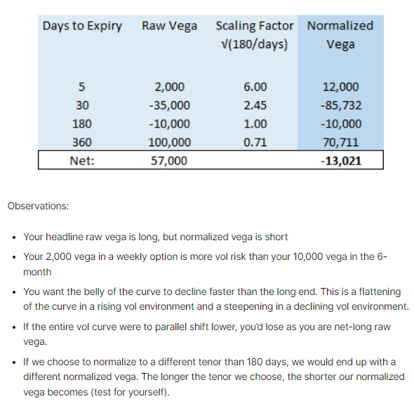
This kind of scaling allows us to summarize the position with a statement like:

“If 6-month vol increases (decreases) by 1 point, I expect to lose (make) $13k”

This would not be obvious if you are looking at the sum of raw vega.

√t scaling is not pulled out of a hat. It corresponds to a world where straddle spreads are constant (again, ignoring theta). Armed with that straddle approximation formula, it is simple to prove that to yourself.

There’s nothing gospel about this weighting scheme. In the moontower.ai app users can view daily vol changes scaled to several choices of tenors. The point is that by normalizing at all, it is easy to see which straddle spreads changed. Implied volatility is a shortcut to get to a price and prices are what your p/l depends on. If you have a time spread on, the change in its price is the thing you care about.

Any vol weighting scheme you choose will not be perfectly accurate (if it were you could literally predict how the vols would change relative to each other, in which case you should have already chucked your phone in the ocean from the hammock of your private island). But it’s a gigantic improvement in risk monitoring from raw vega. Of course, any summary measure is a trade-off between convenience and resolution. The explicit trade-off with √t scaling:

Benefit: Easy to see changes in time spread prices across the term structure. Highly intuitive and interpretable.

Drawback: Inaccurate. Said differently — there’s lots of room to improve the accuracy of the weights from empirical data which will lead to better understanding of vega risk.

Personally, I think dialing in better weights would increase cognitive load. You’ll need to think about what regime or lookback the updating weights are drawn from. The inaccuracies of the constant straddle spread assumption are “the devil I already know”.

[At the risk of wasting digital ink, it should be obvious that designing metrics always depends user context. Building infra and dashboards is an exercise in being a product manager that serves many clients — traders, risk managers, accounting, and back office.]

√t scaling is a meaningful but rough improvement in measuring vega by treating weighting each month differently. Constant straddle spread is an implicit dynamic embedded in the calculation. It’s an assumption. So how do vols across a term structure actually move relative to one another?

Let’s see what we can discover by hackin’ on some data.

Viewing term structure

We are used to looking at charts like this:

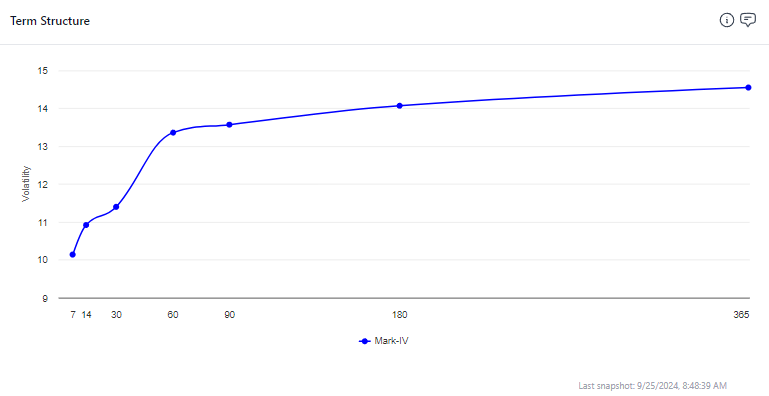
That’s a snapshot of the SPX IV term structure. It’s an ascending shape. We used the term “steepness” to refer to the ratio of 1M/6M vol. In this case it is less than 1.0 since 6-month vol is premium to 1-month.

It’s a common shape (in oil we referred to this as the “droopy penis”). It’s relatively quiet, near vols are subdued, back months expect mean reversion to longer-term averages.

In early August, this would have been sharply descending with a steepness much greater than 1.0 as the near term stress and high realized vol was baked into the front of the IV term structure and sloping down to vols which suggest the markets will eventually calm down.

Instead of a snapshot, a time series can help us capture all that motion. We are going to use about 1 year of GLD data (10/2/23-9/23/24) for the rest of this post.

This is a daily time series of 10d, 30d, 90d, 6M IV. The darker blue line is the 10d IV and the sparkly blue line is the 6m IV. You can see how the 10d IV is itself quite volatile sometimes sagging below the 6m IV (“the droopy penis”) and sometimes shooting way above it into a backwardated or inverted term structure.

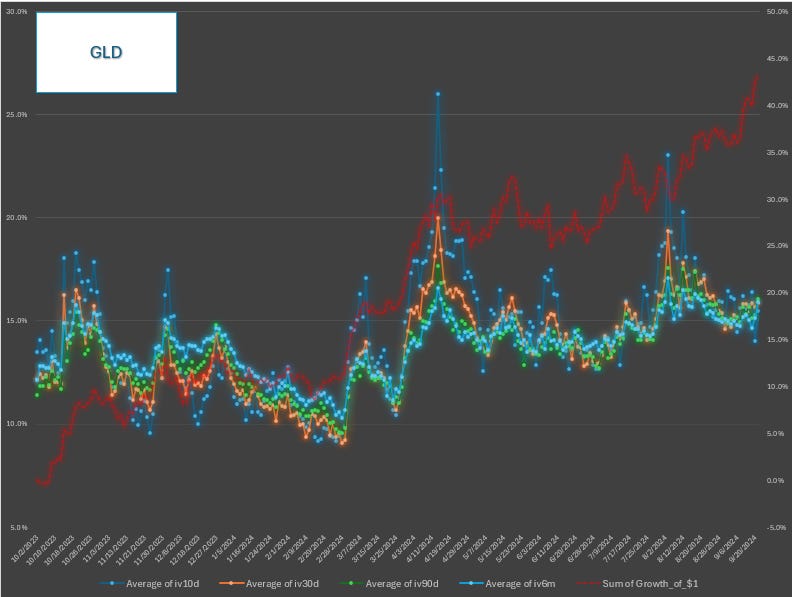
This is an instructive way to see term structure behavior albeit highly zoomed out.

Let’s use another chart for a closer look. We will include 2 time series:

1. The 1M/6M vol ratio
2. The 1M/6M implied forward vol

A forward vol represents the implied amount of volatility that exists between the 1M and 6M expirations. (It sounds complicated but 1 month VIX future settles to “what will the VIX, a 30d forward looking measure, be in 1 month”)

You can use the free moontower.ai forward vol calculator to play with the idea and read about the concept.

The central point is that forward vol is another way to consider the difference in relative volatility between 2 expirations. Seeing things in multiple ways is the focus of this post.

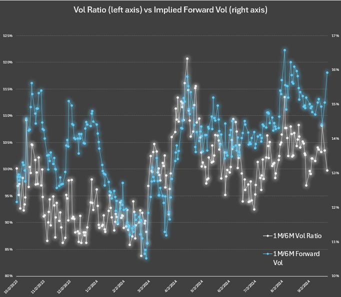
What stands out about this chart?

Here’s what I see:

The forward vol is sometimes high and sometimes low regardless of the ratio.

Let’s say you get an 80 on a test, but there’s a prediction market on your final grade in the class that is trading for 90. The market is implying that you are going to be acing the rest of your tests.

Conceptually the math here is similar — when the front month vol is low and the vol ratio is far below 1.0 (steep term structure) the forward vol can and often does look quite high. The market makes it expensive to lock in cheap volatility for a long time even when the vols are low (the expense will manifest as “roll down”).

But look at early March — not only was the vol ratio low, the forward got crushed. If you only look at vol ratio, you missed this.

Implied forwards are an orthogonal or complementary measure of relative volatility that is additive to your perspective.

I’m a big fan of waiting for imperfectly correlated signals lining up to size up.

Remember, dragonfly eyes.

Next week we will continue with part 2 where we:

• deconstruct the nature of this relationship further
• consider what the differences between lenses means for finding opportunities and measuring risk
• substantiate both the how and why of extending the analysis
  • I plan to actually publish the extended analysis as well, but it won’t fit in next week’s letter on top of the rest of this