Understanding Implied Forwards

These are not trick questions:

Suppose you have an 85 average on the first 4 tests of the semester. There’s one test left. All tests have an equal value in your final score. You need a 90 average for an A in the class.

What do you need on the last test to get an A in the class?

What is the maximum score you can get for the semester?

If you are comfortable with the math you have the prerequisites required to learn about a useful finance topic — implied forwards!

Implied forwards can help you:

• find trading opportunities
• understand arbitrage and its limits

We’ll start in the world of interest rates.

The Murkiness Of Comparing Rates Of Different Maturities

Consider 2 zero-coupon bonds. One that matures in 11 months and one that matures in 12 months. They both mature to $100.

Scenario A: The 11-month bond is trading for $92 and the 12-month bond is trading for $90.

What are the annualized yields of these bonds if we assume continuous compounding?¹
Computing the 12-month yield

r = ln($100/$90) = 10.54%
Computing the 11-month yield

r = ln($100/$92) * 12/11 = 9.10%

This is an ascending yield curve. You are compensated with a higher interest rate for tying up your money for a longer period of time.

But it is very steep.

You are picking up 140 extra basis points of interest for just one extra month.

Let’s do another example.

Scenario B: We’ll keep the 12-month bond at $90 but say the 11-month bond is trading for only $91.
Computing the 11-month yield

r = ln($100/$91) * 12/11 = 10.29%

So now the 11-month bond yields 10.29% and the 12-month bond yields 10.54%

You still get paid more for taking extra time risk but maybe it looks more reasonable. It’s kind of hard to reason about 25 bps for an extra month. It’s murky.

Think back to the test score question this post opened with. There is another way of looking at this if we use a familiar concept — the weighted average.

The Implied Forward Interest Rate

We can think of the 12-month rate as the average rate over all the intervals. Just like a final grade is an average of the individual tests.

We can decompose the 12-month rate into the average of an 11-month rate plus a month-11 to month-12 forward rate:

“12-month” rate = “11-month” rate + “11 to 12-month” forward rate

Let’s return to scenario A:

12-month rate = 10.54%

11-month rate = 9.1%

Compute the “11 to 12-month” forward rate like a weighted average:

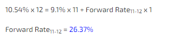
We knew that 140 bps was a steep premium for one month but when you explicitly compute the forward you realize just how obnoxious it really is.

How about scenario B:

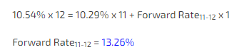
12-month rate = 10.54%

11-month rate = 10.29%

Compute the “11 to 12-month” forward rate like a weighted average:

Arbitraging The Forward Rate (Sort Of)

It’s common to have a dashboard that shows term structures. But the slopes between months can be optically underwhelming with such a view. Seeing that the implied forward rate is 13.26% feels more profound than seeing a 25 bps difference between month 11 and month 12.

You may be thinking, “this forward rate is a cute spreadsheet trick, but it’s not a rate that exists in the market.”

Let’s take a walk through a trade and see if we can find this rate in the wild.

The first step is just to ground ourselves in a basic example before we understand what it means to capture some insane forward rate.

Consider a flat-term structure:

[Note: the forward rate should be 10.54% but because I’m computing YTM on a bond price that only goes to 2 decimal places we are getting an artifact. It’s immaterial for these demonstrations]

Now let’s look back at the steep term structure from scenario A:

With an 11-month rate of 9.10% and a 12-month rate of 10.54% we want to borrow at the shorter-term rate and lend at the longer-term rate. That means selling the nearer bond and buying the longer bond.

When you study asset pricing, one of the early lessons is to step through the cash flows. This is the basis of arbitrage pricing theory (APT), a way of thinking about asset values according to their arbitrage or boundary conditions. As opposed to other pricing models, for example CAPM, someone using APT says the price of an asset is X because if it weren’t there would be free money in the world. By walking through the cash flows, they would then show you the free money². The fair APT price is the one for which there is no free money.

Stepping Thru The Cash Flows

Let’s see how this works:
Today

1. We short the 11-month bond at $92
2. We buy 1.022 12-month bonds for $90. We can buy 1.022 of the cheaper bonds from the proceeds of selling the more expensive $92 bond. The net cash flow or outlay is $0.
3. Spend the next 11 months surfing.

At the 11-month maturity, we will need $100 to pay the bondholder of the 11-month bond so we sell 12-month bonds.

But for what price?

Well, let’s say the prevailing 1-month interest rate matched the rates we were seeing in the flat term structure world of 10.49%, the rate implied by the 11-12 month forward when we initiated the trade.

In that case, the bonds we own are worth $99.13.

[With one month to maturity we compute the continuous YTM: ln(100/99.13) * 12 = 10.49%]

If we sell 1.009 of our bonds at $99.13 we can raise the $100 to pay back the loan. We are left with .0134 bonds.

At the 12-month maturity, our stub of .0134 bonds mature and we are left with $1.34.

So what was our net return?

Hmm, lemme think, carry the one, uh — infinite!

We did a zero cash flow trade at the beginning. We didn’t lay out any money and ended with $1.34.

That’s what happens when you effectively shorted a 26.37% forward rate but the one-month rate has rolled down to something normal, in this case about 10.50%

[In real life there is all kind of frictions — you know like, collateral when you short bonds.]

Summary table:

What if somehow, that crazy 26.37% “11-12 month forward rate” didn’t roll down to a reasonable spot rate but actually turned out to be a perfect prediction of what the 1-month rate would be in 11 months?

Let’s skip straight to the summary table.

Note the big difference in this scenario: the bond with 1 month remaining until maturity is only worth $97.83 (corresponding to that 26.33% yield, ignore small rounding). So you need to sell all 1.022 of the bonds to raise $100 to pay back the loan.

Besides frictions, you can see why this is definitely not an arbitrage — if the 1-month rate spiked even higher than 26.33% the price of the bonds would be lower than $97.83. You would have sold all 1.022 of your bonds and still not been able to repay the $100 you owe!

So the “borrow short, lend long” trade is effectively a way to short a 1-month forward at 26.33%. It might be a good trade but it’s not free money.

Still, this exercise shows how our measure of the forward is a tradeable level!

[If you went through the much more arduous task of adjusting for all the real-world frictions and costs you would impute a forward rate that better matched what you considered to be a “tradeable price”. The principle is the same, the details will vary. I was not a fixed-income trader and own all the errors readers discover.]

The Implied Forward Volatility

Now you’re warmed up.

Like interest rates, implied volatilities have a term structure. Every pair of expiries has an implied forward volatility. The principle is the same. The math is almost the same.

With interest rates we were able to do the weighted average calculation by multiplying the rates by the number of days or fraction of the year. That’s because there is a linear relationship between time and rates. If you have an un-annualized 6-month rate, you simply double it to find the annualized rate. You can’t do that with volatility.³

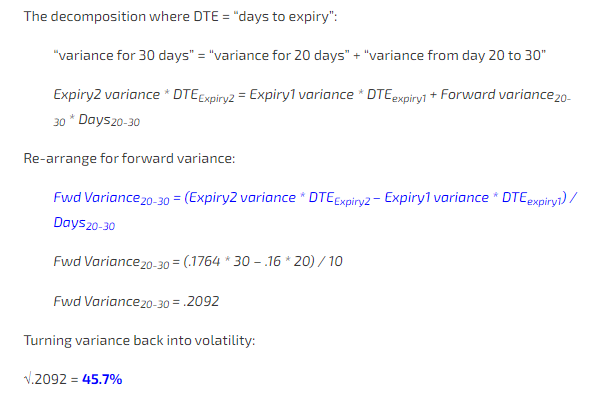
The solution is simple. Just square all the implied volatility inputs so they are variances. Variance is proportional to time so you can safely multiply variance by the number of days. Take the square root of your forward variance to turn it back into a forward volatility.

Consider the following hypothetical at-the-money volatilities for BTC:

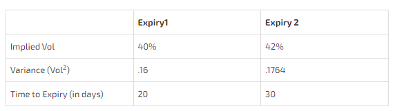
Let’s compute the 20-to-30 day implied forward volatility. We follow the same pattern as the weighted test averages and weighted interest rate examples.

If the 20-day option implies 40% vol and the 30-day option implies 42% vol, then it makes sense that the vol between 20 and 30 days must be higher than 42%. The 30-day volatility includes 42% vol for 20 days, so the time contained in the 30-day option that DOES NOT overlap with the 20-day option must be high enough to pull the entire 30-day vol up.

This works in reverse as well. If the 30-day implied volatility were lower than the 20-day vol, then the 20-30 day forward vol would need to be lower than the 30-day volatility.

The Arbitrage Lower Bound of a Calendar Spread

The fact that the second expiry includes the first expiry creates an arbitrage condition (at least in equities). An American-style time spread cannot be worth less than 0. In other words, a 50 strike call with 30 days to expiry cannot be worth less than a 50 strike call with 20 days to expiry.

Here’s a little experiment (use ATM options, it will not work if the options are far OTM and therefore have no vega):

Pull up an options calculator where you make a time spread worth 0.

I punched in a 9-day ATM call at 39.6% vol and a 16-day ATM call at 29.70001% vol. These options are worth the same (for the $50 strike ATM they are both worth $1.24).

Now compute the implied forward vol.

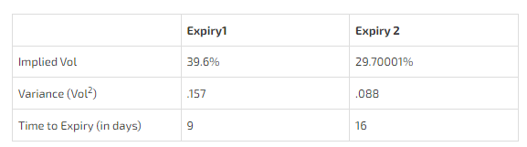
You can predict what happens when we weight the variance by days:

Expiry1 = .157 * 9 = 1.411

Expiry2 = .088 * 16 = 1.411

Expiry 2 has the same total variance as Expiry 1 which means there is zero implied variance between day 9 and day 16.

The square root of zero is zero. That’s an implied forward volatility of zero!

A possible interpretation of zero implied forward vol:

The market expects a cash takeover of this stock to close no later than day 9 with 100% probability.

A Simple Tool To Build

With a list of expirations and corresponding ATM volatility, you can construct your own forward implied volatility matrix:

Arbitrage?

Like the interest rate forward example, there’s no arbitrage in trying to isolate the forward volatility unless you can buy a time spread for zero.⁴

For most of the past decade, implied volatility term structures have been ascending (or “contango” for readers who once donned a NYMEX or CBOT badge). If you sell a fat-looking time spread you have a couple major “gotchas” to contend with:

1. Weighting the trade
   
   If you are short a 1-to-1 time spread you are short both vega, long gamma, paying theta. This is not inherently good or bad. But you need a framework for choosing which risks you want and at what price (that statement is basically the bumper sticker definition of trading imbued simultaneously with truth and banality). If you want to bet on the time spread narrowing, ie the forward vol declining, then you need to ratio the trades. The end of Moontower On Gamma discusses that. Even then, you still have problems with path-dependence because the gamma profile of the spread will change as soon as the underlying moves. The reason people trade variance swaps is that the gamma profile of the structure is constant over a wide range of strikes providing even exposure to the realized volatility. Sure you could implement a time spread with variance swaps, but you get into idiosyncratic issues such as bilateral credit risk and greater slippage.
   
2. The bet, like the interest rate bet, comes down to what the longer-dated instrument does outright.You were trying to isolate the forward vol, but as time passes your net vega grows until eventually the front month expires and you are left with a naked vol position in the longer-dated expiry and your gamma flips from highly positive to negative (assuming the strikes were still near the money).

Term structure bets are usually not described as bets on forward volatility bets but more in the context of harvesting a term premium as time passes and implied vols “roll down the term structure”. This is a totally reasonable way to think of it, but using an implied forward vol matrix is another way to measure term premiums.

The Wider Lessons

Process

Forwards vols represent another way to study term structures. Since term structures can shift, slope, and twist you can make bets on the specific movements using outright vega, time spreads, and time butterflies respectively. A tool to measure forward vols is a thermometer in a doctor’s bag. How do we conceptually situate such tools in the greater context of diagnosis and treatment?

Here’s my personal approach. Recognize that there are many ways to skin a cat, this is my own.

1. I use dashboards with cross-sectional analysis as the top of an “opportunity funnel”. You could use highly liquid instruments to calibrate to a fair pricing of parameters (skew, IV risk premium, term premium, wing pricing, etc) in the world at any one point in time. This is not trivial and why I emphasize that trading is more about measurement than prediction. To compare parameters you need to normalize across asset types.
   
   To demonstrate just how challenging this is, an interview question I might ask is:
   Price a 12-month option on an ETF that holds a rolling front-month contract on the price of WTI crude oil⁵
   I wouldn’t need the answer to be bullseye accurate. I’m looking for the person’s understanding of arbitrage-pricing theory which is fundamental to being able to normalize comparisons between financial instruments. The answer to the question requires a practical understanding of replicating portfolios, walking through the time steps of a trade, and computing implied forward vols on assets with multiple underlyers. (Beyond pricing, actually trading such a derivative requires understanding the differences in flows between SEC and CFTC-governed markets and who the bridges between them are.)
   
2. The contracts or asset classes that “stick out” become a list of candidates for research. There are 2 broad steps for this research.
   
   • Do these “mispriced” parameters reveal an opportunity or just a shortcoming in your normalization?
     
     Sleuthing the answer to that may be as simple as reading something publicly available or could require talking to brokers or exchanges to see if there’s something you are missing. If you are satisfied to a degree of certainty commensurate with the edge in the opportunity that you are not missing anything crucial, then you can move to the next stage of investigation.
     
   • Understanding the flow
     
     What flow is causing the mispricing? What’s the motivation for the flow? Is it early enough to bet with it? Is it late enough to bet against it? You don’t want to trade the first piece of a large order but you will not get to trade the last piece either (that piece will be either be fed to the people who got hurt trading with the flow too early as a favor from the broker who ran them over — trading is a tit-for-tat iterated game, or internalized by the bank who controls the flow and knows the end is near.)
     
3. Execute
   
   Suppose you determine that the term structure is too cheap compared to a “fair term structure” as triangulated by an ensemble of cross-sectional measurements. Perhaps, there is a large oil refiner selling gasoline calls to hedge their inventory (like covered calls in the energy world). You can use the forward vol matrix to drill down to the expiry you want to buy. “Ah, the 9-month contract looks like the best value according to the matrix. Let’s pull up a montage and see if it’s really there. Let’s see what the open interest is?…”
   As you examine quotes from the screens or brokers, you may discover that the tool is just picking up a stale bid/ask or wide market, and that the cheapest term isn’t really liquid or tradeable. This isn’t a problem with the tool, it’s just a routine data screening pitfall. The point is that tools of this nature can help you optimize your trade expression in the later stage of the funnel.

Meta-understanding

This discussion of forward vols was like month 1 learning at SIG. It’s foundational. It’s also table stakes. Every pro understands it. I’m not giving away trade secrets. I am not some EMH maxi⁶ but I’ll say I’ve been more impressed than not at how often I’ll explore some opportunity and be discouraged to know that the market has already figured it out. The thing that looks mispriced often just has features that are overlooked by my model. This doesn’t become apparent until you dig further, or until you put on a trade only to get bloodied by something you didn’t account for as a particular path unfolds.

This may sound so negative that you may wonder why I even bother writing about this on the internet. Most people are so far out of their depth, is this even useful? My answer is a confident “yes” if you can learn the right lesson from it:

There is no silver bullet. Successful trading is the sum of doing many small things correctly including reasoning. Understanding arbitrage-pricing principles is a prerequisite for establishing what is baked into any price. Only from that vantage point can one then reason about why something might be priced in a way that doesn’t make sense and whether that’s an opportunity or a trap⁷. By slowly transforming your mind to one that compares any trade idea with its arbitrage-free boundary conditions or replicating portfolio/strategy, you develop an evergreen lens to ever-changing markets.

You may only gain or handle one small insight from these posts. But don’t be discouraged. Understanding is like antivenom. It takes a lot of cost and effort to produce a small amount⁸.

If you enjoy this process despite its difficulty then it’s a craft you can pursue for intellectual rewards and profit.

If profit is your only motivation, at least you know what you’re up against.

Footnotes

1. We will compute all bond yields under an assumption of continuous as opposed to discrete compounding intervals. If the expression e^rt is foreign to you, I put together this 2-minute post, Examples Of Comparing Interest Rates With Different Compounding Intervals, to demonstrate.
2. I have plans to make a dictionary or taxonomy of the arbitrage relationships in the options world using the cash flow methods to show why those relationships exist. If you’re impatient, Natenburg does an approachable job of this already. His book is how many Wall Streeters learned about them over the past few decades.
3. Volatility is proportional to the square root of time. That’s an annoying thing to say. Instead we can just square the square root of time to be left with time but then we must also square volatility. What’s volatility squared? Variance.If this is confusing, recall that volatility is the same thing as standard deviation. To compute a standard deviation in statistics we first find the variance by:To turn variance into a standard deviation, a number we have intuition for, we take the square root of the variance to undo all the squaring we did in the first place. But when we do that, we also take the square root of variance’s denominator — N.
   1. summing sum the squared differences from each data point to the mean
   2. taking the average by dividing by N
      
      To turn variance into a standard deviation, a number we have intuition for, we take the square root of the variance to undo all the squaring we did in the first place. But when we do that, we also take the square root of variance’s denominator — N.

If we sample volatility daily, N corresponds to the number of days in the sample (for example “close-to-close” volatility). 

4. Also not an arbitrage, but this topic is similar to the concept of “renting a straddle” ahead of earnings. There are situations where a straddle containing earnings is cheap enough that you don’t expect it to decay until the earnings are announced. Re-framing this: the earnings might be fairly priced but the time leading up to earning is being ascribed zero volatility. You could also interpret it as earnings vol is “too low”. Either way, the straddle is not decaying as each day passes, which mechanically means the implied vol is increasing every day by the ratio of theta/vega. For example, if the theta is 2 cents and the vega is 1 cent then implied vol is rising 2 points to keep the straddle unchanged. If the earnings date were also the expiration date, then just before earnings are announced, the implied vol and corresponding straddle would represent a pure market consensus on how much volatility the announcement meant for the stock
5. USO used to hold the front month, then over several days roll into the second month. Since oil went negative in 2020 it holds a basket of futures. One day, I’ll explain a trade I did to exploit mispriced USO vol during that period of time. It had several moving parts and was more of a special situations play than anything else. There was an arbitrage-pricing insight you needed before you could spot it, again, driving home the importance of this thinking generally.
6. I’m allergic to academic discussions of EMH. I prefer to say there are no easy trades. 
7. An example of a trap: What The Widowmaker Can Teach Us About Trade Prospecting And Fool’s Gold
8. From Wikipedia: Antivenom is traditionally made by collecting venom from the relevant animal and injecting small amounts of it into a domestic animal [like a horse]. The antibodies that form are then collected from the domestic animal’s blood and purified.