the 2 vectors of volatility scaling

I fired up Corey Hoffstein’s goated Flirting With Models podcast to hear Scott Phillips discuss “ugly” edges in crypto. This episode came highly recommended in my corner of twitter. It does not disappoint.

But I want to zoom in on one part. Scott says:

If you did what I do perfectly, you'd be up well over Sharpe two, and probably with size. But the way that I do it, our four-year Sharpe is 1.7 with retail-level costs. So cross-sectional momentum is a little bit better than that, but you don't have the really nice positive skew of trend. And cross-sectional carry is about a Sharpe 1.7 as well, and slightly orthogonal. So you blend the three of them together, and then you're at Sharpe two easily — and without even good execution…The math holds. Returns scale with the square root of independent bets.

Scott misspeaks here (easy to do in a conversation) but what Scott means is volatility scales with the square root of independent bets (returns scale linearly). This concept underpins one of my most important posts — Understanding Edge. It is the basis of all trading businesses without exception. It’s Day 1 learning at a prop shop. Munger has that “Take a simple idea and take it seriously” advice…This is THE idea Jeff Yass took seriously.

I’m repetitive on log and compounding math for 2 reasons that extend beyond the shock factor of the “lilypads in a pond” puzzle:

a) Investing is a serially repeated game so compound returns are our primary concern

b) Option theory sits atop logreturn math which is just continuous compounding (in fact e, the Euler constant of 2.718, is your growth of $1 if you continuously compound at 100% rate for 1 unit of time. See Using Log Returns And Volatility To Normalize Strike Distances)

We’ve confronted this math many times from different angles:

• The Volatility Drain
• Path: How Compounding Alters Return Distributions
• Examples Of Comparing Interest Rates With Different Compounding Intervals
• Well What Did You “Expect”?
• Geometric vs Arithmetic Mean In The Wild
• Understanding Log Returns
• I Felt Bad For Picking My 3rd Grader Off
• Getting Comfortable With Log Charts
• you can ONLY eat risk-adjusted returns
• Growth rate = 70% * (doublings/years)

Compounding is a multiplicative process that describes how returns scale across time. “Volatility drain” reminds us that volatility’s interaction with growth is embedded in that process.

We already understand how compounding scales across time as a function of volatility.

But volatility itself has scaling properties.

That’s what Scott means when he says (or meant to say) it grows by the square root of independent bets. Regular readers have seen me scale a daily return to an annual return by √251 or ~16 many times. But I don’t always remember to say that this assumes no correlation between daily vols (mapping to the “independent bets” language).

In multiple posts, we have seen that volatility is understated in the presence of autocorrelation:

• Thinking in N not T
• Volatility Depends On The Resolution
• the option market's point spread (part 2)

Autocorrelation affects how we scale vol through time per asset.

This is only half the volatility scaling story. It’s one vector.

The second vector is how we scale vol across our portfolio.

This depends not on autocorrelation, but on pair-wise correlation.

Independent bets are simply bets that have no (ie zero) correlation with one another.

It is why you can blend several strategies and end up with a composite Sharpe greater than any of the components.

Let’s look closer.

Let’s consider an equal-weighted portfolio of ETFs:

• IBIT (BTC)
• GLD (gold)
• HYG (high yield credit)
• IEF (10-year notes)
• QQQ (Nasdaq stocks)

Method:

1. I used the hedge ratio tool to fetch the correlation of daily returns for each of the 10 possible pairs (5 choose 2) for the past 16 months.
2. I chose a reasonable vol for each name and then backed out an expected return by assuming the Sharpe Ratio of each asset is .40. I’m ignoring RFR in SR — I’m just using expected return / vol.
3. I convert the correlation table into a covariance table to do the matrix multiplication for computing portfolio vol. I explain the math in writing, video, and in a spreadsheet I’ve shared before:
   1. ✍🏽Computing portfolio vol (moontower)
   2. 🔻 Portfolio Vol Spreadsheet (download)
   3. 🎥Portfolio Vol Explainer (Moontower YouTube)

Here’s my work for the equal-weighted portfolio:

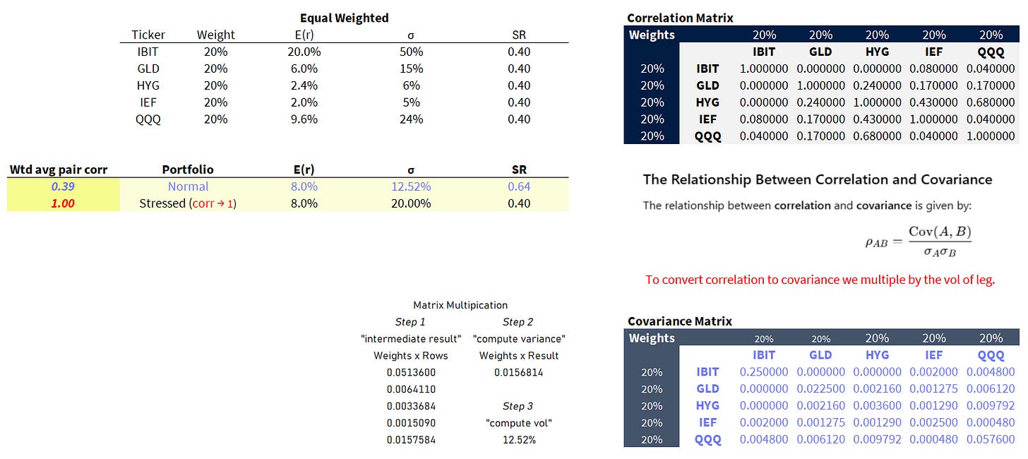
What to take note of:

• If we compute the portfolio vol in the “stressed” condition where all the pair-wise correlations are 1.0, then the portfolio vol is equal to the weighted average vol of the components. In this case, the portfolio vol is 20%. There’s no diversification benefit to the portfolio vol or SR!
• When we use the actual correlations the portfolio vol drops to 12.5%. Since the expected return is unchanged the SR improves from .4 to .64. Massive diversification benefit.
• The ratio of the portfolio variance to average weighted stock variance is the average weighted pair-wise correlation. The average weighted stock variance is the same as the portfolio variance if all the correlations are 1.0
  • For the option fans: this math is exactly how implied correlation is backed out of the index option market. The ratio of index variance to weighted average stock in the basket’s variance is the implied correlation! The cheaper index vols are relative to stock vols, the more implied diversification benefit there is in the index. This concept sits at the heart of dispersion trading.

A portfolio that equal weights IBIT and IEF sounds a bit comical. Let’s re-do the analysis with an inverse vol-weighted portfolio:

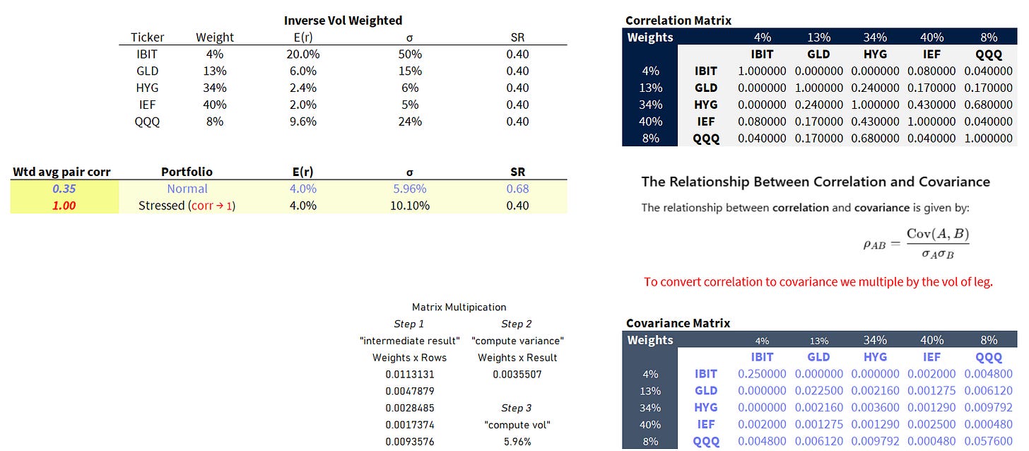
Now IEF has 10x the weight IBIT does. If you multiply each component’s weight by its vol you’ll notice they each have equal risk contribution.

The normal portfolio has a Sharpe of .68 but if all corrs go to 1.0 the SR drops to .40 and the portfolio vol goes from 6% to 10%.

Even if the math isn’t interesting, the principle should be seared into your risk brain. Adding zero or negative correlation assets to a portfolio can improve its risk/reward even if the asset’s individual SR is inferior to the average component. An asset’s stand-alone properties are not as important as how it contributes to the risk/reward of your portfolio just as how an asset’s arithmetic return does not mean much if don’t consider its vol. After all, we care about compounded returns.

These dual concepts, timer-series volatility (influenced by auto-correlation) and cross-sectional volatility (influenced by pair-wise correlation of components) give a fuller picture of how returns AND volatility accumulate through time. You care how both the numerator (return) and denominator (risk) scale.

Application to allocators

Professional allocators recognize that much of the low-hanging fruit of long-term results is sound portfolio construction. Basic hygiene in how you stack investments by understanding their properties in various states of the world is something you have more control over because volatility and correlation are more stable than expected return predictions. Simple optimizers are incredibly sensitive to expected returns — which is a bit self-defeating when you realize this is the metric we know the least about.

To add a bit of practical color. I have a good friend — a physics academic turned investor — who was CIO for the family office of one of the partners of [insert the best quant firm you’ve heard of and it’s probably the one]. He admit something he found embarrassing — a shockingly small number of ideas underpinned the family office’s approach and none of them is a secret. The scaling property of portfolios is one of them. If they sourced 16 investments that generated a high-quality portfolio, in order to double the shape they needed 4x as many additions to that portfolio of similar quality (which was already high) to double the portfolio Sharpe. Pretty much impossible when all the investments are LP stakes in quant funds (due diligence alone is too labor intensive, never mind finding that many great managers).

[I’ll get around to toying with this tool a bit more to tinker my way to seeing how the scaling works — for example going from a 3 stock to 12 stock portfolio where I add names with equal SR but different correlations. I’m down to the wire on writing this post as it is.]

Application to traders

The last part of this video shows how the interaction of return and volatility can inform how you think about sizing risk.

If you prefer text, the heart of the material is captured here:

Understanding Daily vs. Annual Sharpe — and Sizing Risk with Intent

Let’s start with something simple but important.

🗓 Daily SPX Returns

The S&P 500 has a daily mean drift of about 3 basis points, with a standard deviation of about 100 basis points in normal conditions. That gives you a:

Daily Sharpe ≈ 0.03

(This ignores the risk-free rate, which is roughly 1.5 bps/day.)

📆 Annual SPX Returns

Now zoom out.

The S&P’s annual return is roughly 8%, with an annualized volatility of 16%. That gives:

Annual Sharpe = 8 / 16 = 0.50

Here’s the interesting part:

Annual Sharpe (~0.50) ≈ 16× Daily Sharpe (0.03)

Why? Because volatility annualizes by the square root of time:

√251 ≈ 15.8, or roughly 16

🎯 Sharpe Ratio Benchmarks

Let’s anchor a few examples to make this more intuitive:

• SPX benchmark: 3 bps return / 100 bps vol → Sharpe 0.03
• Sharpe 16 strategy: 1% return/day, 1% vol/day → Sharpe 1.0 daily
• Sharpe 2 strategy (annual) =
  → Daily Sharpe ≈ 2 / 16 = 0.125

So:

A Sharpe 2 strategy means your daily standard deviation is ~8× your expected return.

That 8-to-1 ratio is a helpful sanity check.

💰 Backing Into Risk Limits

Let’s say you want to size your book around a Sharpe 2 strategy. Here’s one framing:

• Daily P&L target: $1,000
• Daily volatility: $8,000
  → Daily Sharpe = 0.125
  → Annual Sharpe = 2.0

Now annualize:

• Yearly expectancy: $1,000 × 251 ≈ $251,000
• Annual volatility: $8,000 × √251 ≈ $126,744

What does this imply for annual ranges?

• A +1 SD year: $124,256 – $377,743
• A +2 SD year: ~0 – $500k
• You're brushing against zero at 2 SDs

📐 How to Use This for Book Sizing

You don’t just ask how much do I expect to make?

You ask:

• What kind of daily swings are consistent with my goals and risk tolerance?
• Can I size positions and set Greek tolerances so that my volatility lands near ~8× my expectancy (for a Sharpe 2 strategy)?
• Do I have enough emotional and capital runway to survive the downside scenarios?