On Jan 28th, one of my favorite topics came up in the Moontower Discord: natural gas options!

I was asked why the VRP was so low.

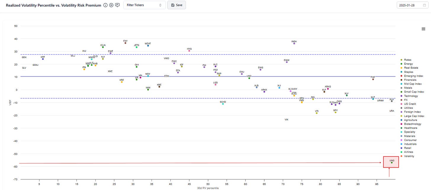
Recall VRP is the comparison of implied vol (forward looking) to realized vol (backwards) looking. In this datapoint,

One month IV = 49%

One month RV = 86%

The strange datapoint is a perfect icebreaker for discussing:

• seasonality (which happens to be most strongly expressed in natural gas)
• a common pitfall (and potential correction) for VRPs

Background

Before discussing options, we need to understand the shape of seasonality and the fundamentals that drive it. I’ve said many times that I’m not a fundamental trader. That means I don’t position based on any views about fundamentals. But a basic understanding of fundamentals is necessary to make sense of why an asset’s vol surface looks the way it does.

Let’s begin…

A Brief Primer on Natural Gas Dynamics

Natural gas prices follow a seasonal cycle, with volatility peaking in winter due to heating demand and spiking again in summer due to electricity consumption.

Seasonality volatility

Winter is the most volatile season.

• Heating demand: Cold weather drives demand
• Supply constraints: Limited storage or pipeline capacity can trigger price shocks.
• Weather uncertainty: Forecast swings can cause sharp market reactions.

Summer is the next most volatile season.

• Electricity demand: Power plants burn more gas for cooling
• Hurricane season effect on supply: Storms in the Gulf can disrupt production

The Storage Cycle

• Injection Season (April–October): Gas is stored for winter, with October marking peak supply. If storage maxes out, prices can collapse.
  
  [In 2009, this was a major risk with the Oct $2.00 put price surging to an insane vols on extremely heavy volume. I remember feeling terrible for leaving my business partner to deal with that expiration on his own because I had to be in Mexico for my wedding week. He was able to join the festivities after making sure we weren’t going to need a cave to take delivery. I distinctly remember computing that the stretched IVs still never reached the extreme levels of realized vol that accompanied that expiry. On a hedged basis, every option except the ones where Oct gas expired were a buy. The market found the path of maximum pain.]
  
  Injection season is often traded as a package of futures of options known as the “J-V strip” based on their futures month codes. In trader language, the “ape-oct strip”.
  
• Withdrawal Season (November–March): Stored gas is used to meet demand, with March marking peak depletion—low storage levels can drive price spikes.
  
  This season is also traded as a package — the “X-H strip” or “Nov-March”
  

…which brings us to the “widowmaker”.

March-April Spread: A Market Tightness Gauge

The March-April futures spread more affectionally known as the “widowmaker” or simply “H/J”:

• High March premium: Indicates low supply and potential scarcity.
• Weak or negative spread: Suggests ample gas and lower risk.

I’ve written at length about this spread and the options on it.

🔗What The Widowmaker Can Teach Us About Trade Prospecting And Fool’s Gold

You can learn a lot from its vol surface that can be applied to any asset with a “bubble” distribution. Moontower’s ever-so scientific definition: a price that most likely collapses but can reach any arbitrarily high price before it tanks.

🔗What Equity Option Traders Can Learn From Commodity Options

Supporting evidence in pictures

Exhibit A: Natural Gas Inventory 5-Year Seasonality Chart

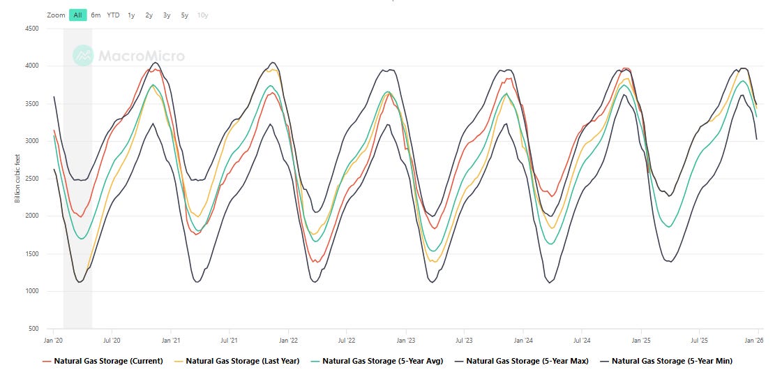
Exhibit B: A historical snapshot of the gas futures term structure

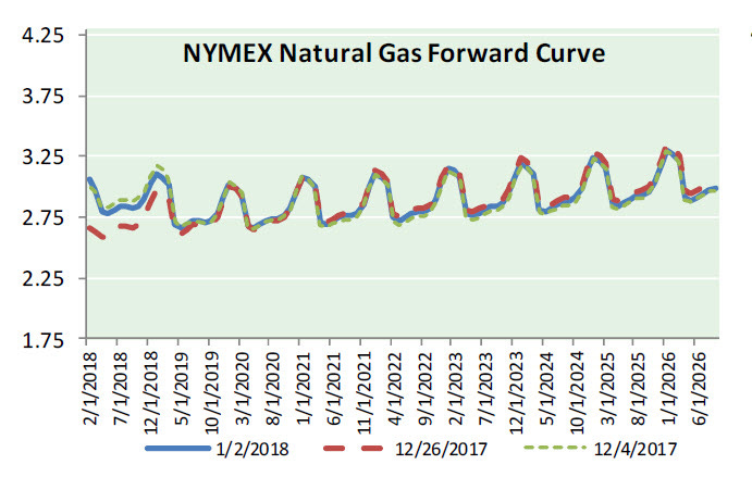
Exhibit C: Realized vol by month

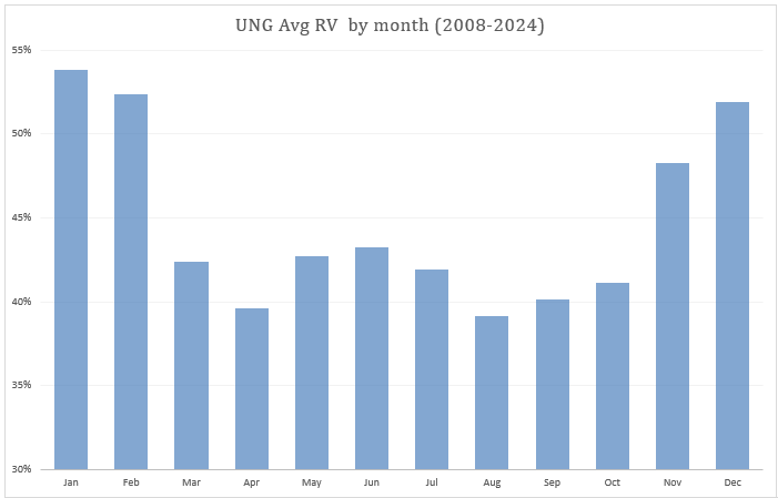
Exhibit D: Despite the strong realized vol seasonality the range of volatilities both across and within years is itself quite volatile.

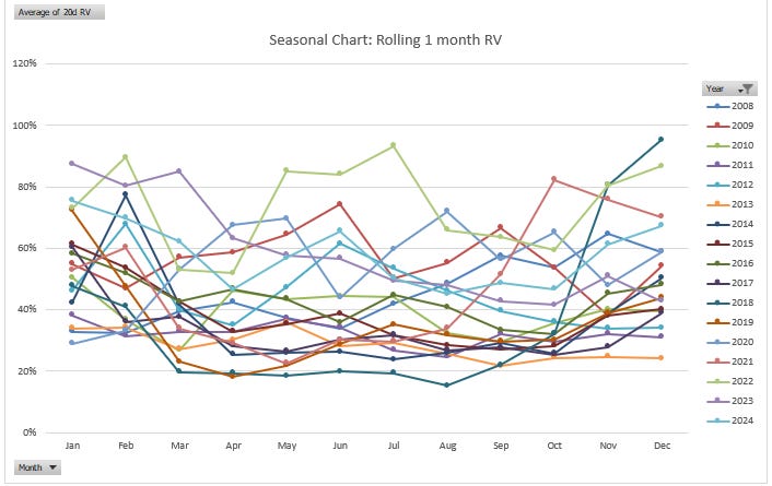
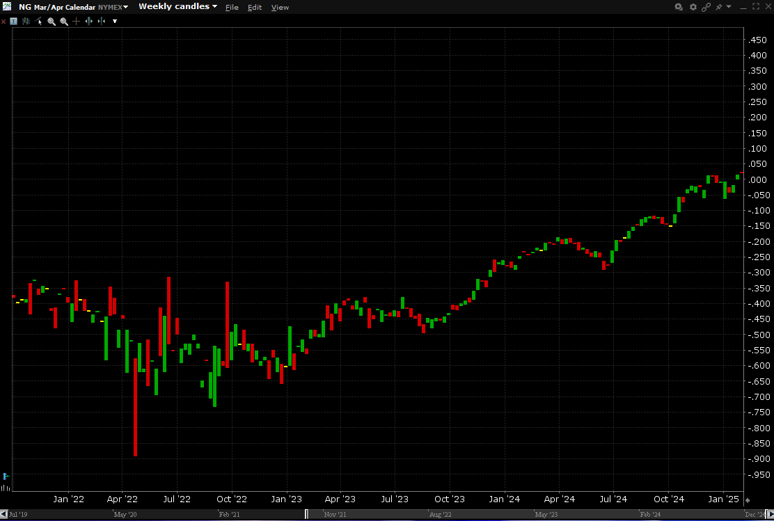
Exhibit E: The March/April futures spread

The “widowmaker” expires this month. In commodity land, futures spread are usually quoted as near month - back month. So in a backwardated market the spread would be positive (ie March > April).

In equity markets the convention is reversed. The price is quoted as back month - front month. The charts below are from IB which uses equity market convention.

You can see the “winter premium” come out of the spread as April is now trading close to parity with March but the spread was negative (ie April < March for the past several months).

This is typical behavior. The spread usually goes to parity as the fear of a cold winter subsides. But it’s dangerous to short early in the season because the spread can go extremely negative (if you’re looking at the price using the IB quoting convention…which burns my eyes but whatever).

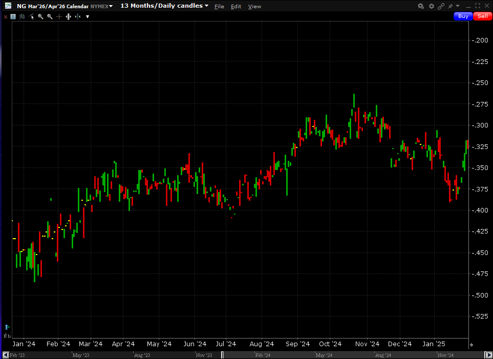
Here you can see the spread for 2026. April is trading at about a 32 cent discount to /March (~10%). If next winter is mild, you’d expect the gap to close.

In the below charts we respect tradition by using the quoting convention of March - April…you can see the destination of the spread is usually ~ 0:

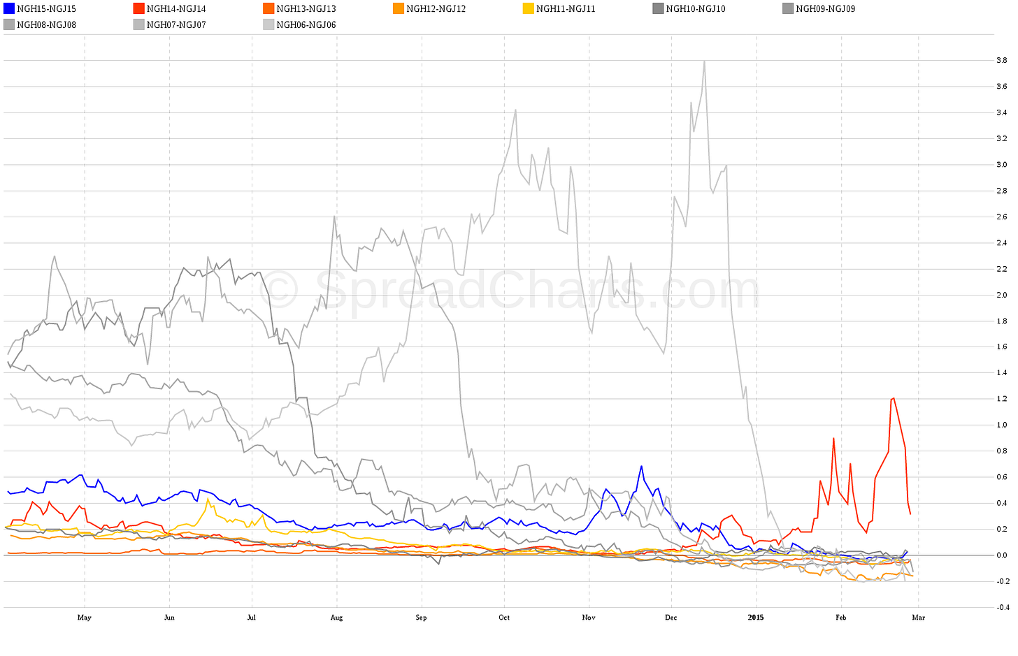
This was the spread in 2007 when John Arnold became a legend stuffing Amaranth’s Brian Hunter’s attempt to squeeze H/J:

Option surface dynamics

Let’s see how these fundamentals influence the vol surface.

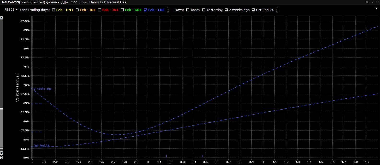
Skew Feature

🔀Inverted skew

Call IVs typically trade at premiums, often steep premiums to puts. Because gas is prone to squeezes it often maintains a “spot up, vol up” dynamic. On the downside, gas can find incremental demand via “coal-switching” whereby gas prices become competitive with coal as a input to electricity generation. This source of demand dampens vol as futures fall reducing the probability of a complete collapse in an oversupplied market.

This is a chart of Feb gas options (note that Feb options expire in January…in commodities the contracts are named after their delivery month not their expiry month). The curves represent roughly 2 weeks and 3 months to expiry. You can see the skew inversion.

💡Learning moment: Note how skew looks steepens when DTE is smaller. Much of this is an artifact of the X-axis being in strike space not delta delta space. Why does that matter? Because how “far” a strike is depends on time. If gas is $3.00, then the $3.20 strike is much further (ie lower delta) with 2 weeks to go than 3 months to go. Low delta options usually command premium IVs.

Term Structure Feature

📅Seasonality in the forward vols

We know that realized vols are higher in the Winter. Look at the vol term structure I pulled from the futures options via CME.

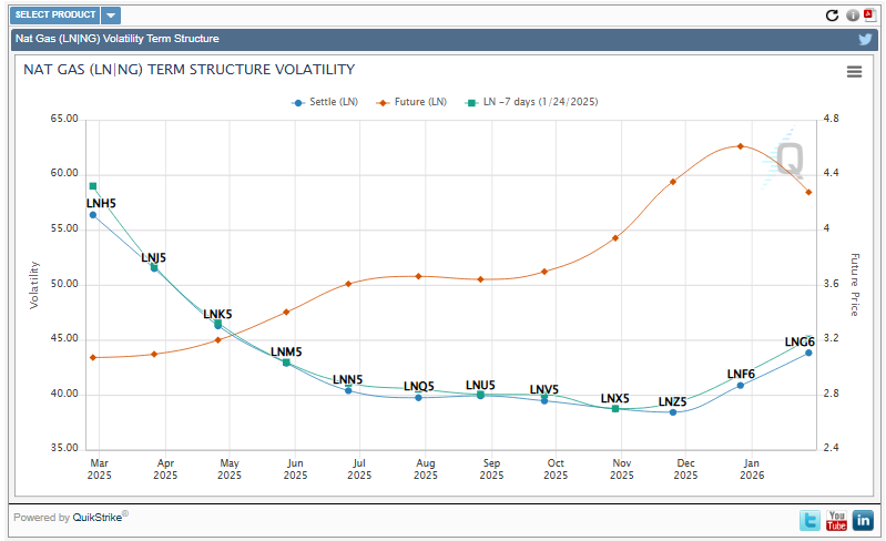
2 things to note:

1. LNF6 and LNG6 slope upwards indicating a higher volatility than Q42025 vols. This makes sense those 2026 capture December and January coldness while LNZ5 December options only capture through Thanksgiving. This tracks, nothing weird.
2. Those winter vols implied vols are LOWER than Spring 2025 vols (ie LNK5 or May). What the heck?!

You have 2 forces colliding from opposite directions.

a. We absolutely expect vol to be higher next winter than this spring

b. Deferred futures contracts don’t move as much as prompt ones.

In other words, the beta of those winter contracts to whats happening now is low. Today’s supply/demand balance for gas has only modest impact on future prices. This is actually a universal effect in commodity futures. This is easy to deomonstrate if we consider a long duration between contract months.

The price of oil today has little impact on what the 5-year future does. Which makes sense. Near term drivers of oil could be weather, refinery outages, shipping logistics, and the current economy. Longer term, oil prices depend on drilling projects, regulations, and the state of economy which is anyone’s guess from our current seat. A price spike today, can lead to more investment in oil, which would increase supply in the future. Nobody thinks that a near term squeeze should have an equal response in the deferred month.

The quantitive observation that deferred months have lower realized than near months is called the Samuelson effect. Stated otherwise, contracts become more volatile as expiry approaches

💡This is a strong effect as a contract travels from being a 12 month contract to a 1 month contract but effect is smaller as a contract goes from being 10-years to 9-year or from 20 days to 1 day. The schedule of how variance decreases as DTE increases looks like a curve. Hold this thought.

The stronger the Samuelson effect, the more downward sloping you’d expect the term structure. The fact that the deferred months are only slightly lower vol and the curve is flat actually implies an ascending term structure if you adjusted for Samuelson effect.

The schedule of how Samuelson unfolds has a tremendous impact on what you believe the term structure actually says. If there was zero Samuelson effect, then the term structure you see is the actual term structure which you are then free to extract forward vols from. That’s the case of equities where all the options are struck on the same underlying as opposed to each expiry referencing a different deferred future.

The stronger the Samuelson effect, the more true term structure and forward vols ascend. If your 1 year future trades at the same implied vol as your 1 month future despite the fact that the 1 year future is moving less, means that the market is implying more variance in the coming months. If there was no Samuelson effect than you’d assume a flat forward vol not an ascending one.

Armed with this knowledge, I present the UNG vols.

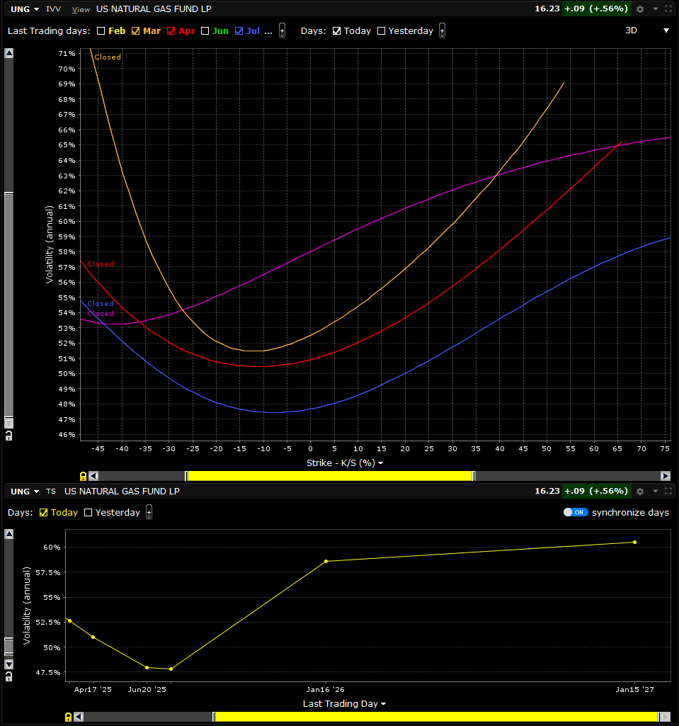
The bottom panel shows UNG vols ascending thru 2025, not descending like the futures options were.

UNG options are struck on a single underlying just like regular equity options, but that underlying ETF maintains exposure to the front month natural gas futures.

In the futures options, the January expiry references a deferred future and expires in December. It is an option that references a contract that will not be moving very much for the next few months, but will be whipping around like crazy near the end of its life.

The January UNG option is referencing a prompt future that moves around a lot and will converge to the futures option in the month of December when the ETF is holding the same contract January futures option references.

The key to translating the futures options vol into a UNG equivalent vol is a schedule for the Samuelson effect. This creates a model that allows market makers to relative value trade the futures options vols vs the ETF vols. (This was central to my strategy which required normalizing commodity vols into something that can be coherently compared to other vol surfaces).

Some food for thought:

✔️Instead of designating a Samuelson schedule, you can invert the problem. What Samuelson schedule needs to be true to make futures options and UNG options be relatively in-line?

✔️How does that schedule compared to how vol unfolded in prior years?

✔️In what ways is the fundamental context of this year different from prior years?

I’ll close this section with one more picture.

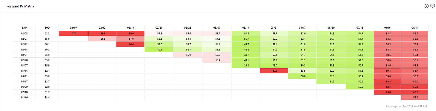
That is the forward vol matrix from UNG courtesy of moontower.ai on 2/4/2025

Recall this chart:

Winter vols average in the low 50s. The forward implied vols are pricing upper 50s. That is a normal premium and if you track the forward vols every day you’ll notice that winter vols 6-12 months out will price somewhere between mid 50s to mid 60s in the case that the upcoming winter supplies look tight.

💡Winter volatility is right-skewed so if the realized avergaes low 50s the median can be assumed to be lower but sometimes the vol is much higher than the 50s. You can see the “polar vortex” in Feb 2014. You can also see just how low the vol can be in the winter:

That chart shows how deferred forward vols are like fair point spreads but have giant error bars compared to the range of realized outcomes.

Additional thoughts

✔️Circling back to the question that launched the post: why was the VRP (ratio of IV to realized vol) so low on January 28th?

Like looking at VRPs after earnings it’s an instance of a VRP failure mode — you are comparing a forward-looking numerator to a backwards-looking denominator. As we change seasons, nobody expects the recent bout of volatility to repeat in the next month.

✔️An example of a trade I did in the mid 2010s

I don’t remeber the exact year but in the early spring, summer vols were getting smashed as producers were selling calls as part of large hedge programs, They were bombing summer call strips. For example, if they sell 5,000 J-V $5 calls they are selling 5,000 calls in each of April, May, June, July, Sep, Oct.

30k call options in total.

I don’t remember how many total calls were sold or how long the program lasted but at some point the vols looked quite tasty.

I eyed July 4 calls which a broker was offering for 10 ticks. 10 ticks = 1 penny. So to breakeven gas had to go to $4.01

A natural gas tick is worth $10 so each option cost $100. I bought 10k for $1mm of premium. Gas was trading in the low $3 range at the time. I decided the best way to manage the trade was to risk budget it instead of delta hedge it. The options were a very cheap vol but I didn’t want to invite the path risk of selling deltas on a grinding rally where a summer risk premium started to emerge if it was looking like a hot season. Instead, I would play for a spikier move. I remember pulling up some historical charts and figuring based on an admittedly low sample size that the chance was somewhere around 20% but if it happened I’d conservatively make 9-1 on the calls. I also asked some sell-siders about whether there was anything in the fundamental context that differentiated this year from prior years.

[There’s a concept I call “analog” years where some years look like others. “In 2007 corn plantings were at this stage by this time of year and everyone thought that summer was going to be hot and the vol surface liked like this”, etc.

I didn’t check on these things so much to ideate a trade as to just check if I was missing something baked into the common knowledge the underlying market when I’m reacting to a trade.]

All told, it was reasonable to risk $1mm in premium, all-or-nothing.

So did the calls hit?

No. But, I was right about the vols being low. It was still early spring and the futures weren’t going anywhere, but the calls stayed penny bid for the next month. A month elapses, spot goes nowhere which means the IV on the strike clearly increased.

From there I had choices, I could re-asses if I thought the vol was still cheap. If not I could roll the calls up, or sell some closer-to-ATM vols and still be long vol-of-vol. If I thought the vol was still seasonally cheap, I could roll them down and have more gamma as the futures started to roll up the Samuelson curve (ie move around more). The point is there was a new set of decisions but they have nothing to do with the original trade which was “buy the cheap vol, decide how to manage it”.

In the end I was right but didn’t make a sum of money that stands out in my memory. This is not especially unusual. Trading be like that.

Extensions to think about

✔️Earnings seasonality

Market-maker’s starting point for thinking about earnings straddles will be:

1. How much has the stock moved on prior earnings dates
2. How was the earnings straddle priced going into those dates

I expect they also consider earnings seasonality. If a retailer makes most of its money in Q4 then the process for pricing earnings won’t be uniform every quarter. The sample size of relevant earnings history will be even smaller as each year maybe there’s only 1 day that is a true analog for appreciating how many days of volatility should be baked into the earnings straddle.

I’d totally expect that the market handles this well. I’m just relating the idea of seasonal volatility to assets outside commodities.

✔️Ags and softs

It’s not surprising that I took the nat gas framework and pointed it at cotton, cocoa, sugar, coffee, soybeans, corn, and wheat. Each of these markets has its own idiosyncrasies. Examples:

• peculiar option to future expiry mapping
• seasonality drivers
• concepts like “old crop” vs “new crop” which means Samuelson curves are discontinuous
• import/export features => currency correlation considerations
• unique natural flows

As a vol trader you are doing some mix of modeling and qualitative adjustments to estimate the implied forward vols in these markets.

💡It’s critical to understand how the distribution of variables that roll up to those numbers effect how the forward vol estimates are distributed…the weaker you think the Samuelson effect is the more you will be inclined to buy time spreads. Are you buying time spreads while your modeling of Samuelson is on the low end of its range? Then realize that your position is more vulnerable to near term stress than your headline greeks would suggest.

If you use percentiles to measure skew, vol or any other metric are you conditioning them on season?

Would it make sense to condition on the degree of backwardation or contango in the market?

Ok, I’m going to leave it there.

If you are interested in commodity vol stuff either directly or just to expand your own option-thinking toolbox check out:

• What Equity Option Traders Can Learn From Commodity Options (13 min read)
• Crossing The Commodity Chasm (13 min read)
• Financial Hacking: ETF vs Negative Oil Futures (a step-by-step explorable)