Pricing 0DTEs

On the last day of November, Kevin bought a bunch of cheap SPY options about 10 minutes to the close and scored. Trades:

Looking at this prompted me to write this post which I’ve had on my mind for a long time: how to think about 0DTEs (or from the bulk of my historical experience — options on the last trading day).

The moontower.ai uses a “volatility lens” for discernment in the option market. But we don’t have a suite of tools for analyzing 0DTE. If we did, we would use a different approach than we do for options broadly. (I’m nothing if not opinionated about how to think about options and being opinionated is part of what you pay for.)

I’ll give you a hint. To think about 0DTEs properly, you must think about time. Any consideration about “vol” can easily be swamped by what you assume about time.

I’ve written about time in options before:

• understanding variance time
• If you annualize volatility with 252 days can you use that number in a 365-day option model?
• weekend theta
• the dirties are down the cleans are up

[The closest hint as to what we’re going to build on was a birdie asked how to model a 1-day option]

But these articles do not address intraday time decay. Option theta is large on the last trading day, while vega is small. 0DTE option pricing is far more sensitive to “How much time remains until expiration?” than notions of volatility.

But the question of how much time remains until expiry is not so simple. Without a concept for how much time remains, we can’t appreciate whether Kevin’s trade was a lucky outcome or strong ex-ante decision.

We’ll unpeel the problem, and in doing so, you’ll get a new view into 0DTE prices.

The most effective way to do this will be to build from a naive model of time passage to a more realistic one to see how it influences option values.

Note: This topic just got way more timely (pun most definitely intended) in light of the Nasdaq’s SEC bid to increase trading hours to 23 hours per day.

Setting the scene

• We are looking at options on our stylized friend, the $100 stock with a 16% vol (corresponding to an expected ~1% daily standard deviation).
• The options are American-style and expire Friday at 4pm.

It’s currently Thursday at 4pm. There is 1 DTE.

Let’s establish a few starting measures. The calculations used in the tables that follow will use the same process.

What’s the $100 straddle worth?

Using our handy approximation:

straddle = .8Sσ√T
straddle = .8 x 100 x .16 x √(1/365)
straddle = $.67

What’s the vega of the straddle?

Straddle vega is defined by change in straddle price per 1 point change in vol. We just rearranged the formula:

vega = straddle/σ = .8S√T / 100
vega = .8 x 100 x √(1/365) / 100
vega = $.042

What’s the 30-minute theta of the straddle?

This is where we need to think differently. If the stock goes nowhere in the next 24 hours the straddle goes to zero. It decays 67cents. But this is far too blunt of a measure if we are trying to think about pricing an option intraday. It’s not illuminating nor useful for our aperture. So we sprinkle in judgment. We’re going to compute a 30-minute theta. There is nothing special about 30 minutes, but you’ll see that just selecting a shorter theta window allows us to reason about time’s relationship to the price of the straddle, and we already hinted that this is the most important driver of price.

We don’t need Black-Scholes. We can compute the theta numerically by pricing the straddle in 30 minutes and taking the difference. If 1 DTE corresponds to 24 hours, then 23.5 hours corresponds to 23.5/24 or .979 DTE

straddle in 30 minutes = .8 x 100 x .16 x √(.979/365)
straddle in 30 minutes = $.663

30-minute Theta = straddle now - straddle in 30 minutes
30-minute Theta = $.67 - $.663  $.007
30-minute Theta = $.007

The naive and invisible assumption

To say that 24 hours equates to 1 DTE and 23.5 hours equates to .979 DTE assumes that “volatility time” passes at the same rate as “wall time” (it’s called “wall time” because clocks are on the wall).

But volatility passes unevenly. Sometimes in bursts. Think of earnings or Fed announcements. The straddle decays instantly after the news is out. Mechanically, traders “crush the vol” in their model to simulate this, but traders on Friday also do things like keep their vols the same and “roll their dates” forward. These are pragmatic kluges to imperfect models to account for the fact that vol does not pass uniformly with time.

[That concept is covered thoroughly on an interday basis in the articles I link to above, but we are zooming in to intraday in this post.]

Our calculations assumed time passes uniformly. Let’s extrapolate the calculations to see what that looks like:

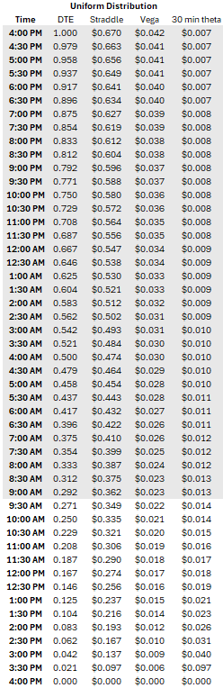
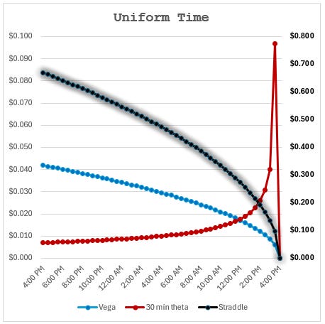
Observations from the uniform time passage assumption

• Theta increases as we approach expiry making the straddle decay faster towards the end of the day
• The straddle’s sensitivity to vol (vega) becomes smaller than 30-minute theta by about noon New York time.

Implication

The value of the straddle is quite sensitive to how much time remains. As we get closer to expiry, it’s clear that even a difference of 10 minutes in your assumptions of how much vol time remains is worth several volatility points.

If market participants understand that time does not pass uniformly, their opinions about the cheapness and expensiveness of the straddles will vary at any singular point of time even if they all agree that the straddle was worth $.67 with 1 DTE!

Differences of opinion are the basis of trading. If you measure time naively, you are a sitting duck for someone who models it better and can buy/sell from you because you are mispricing the “rent” for the next X hours. Of course, this is all masked by 0DTEs by nature having noisy outcomes, but I assure you this is a casino market-makers like being the croupier in.

Towards better time assumptions

From non-linear to the “U-shape”

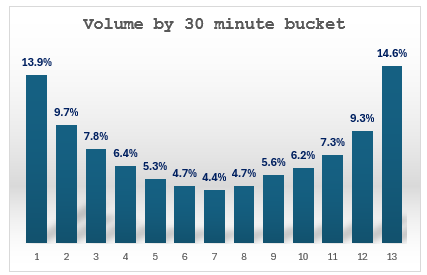
It is widely understood that market volumes are not uniform throughout the day. The opening and closing 30-minute periods punch above their weight out of a 6.5-hour trading day. VWAP algorithms, which target the day’s “volume-weighted average price”, send child orders in proportion to the day’s volume signature rather than slicing the order evenly throughout the day.

It turns out that this volume profile is strongly linked to the intraday volatility profile. That’s what we care about for pricing options. While unexpected news can change the value of assets without any trading occurring (a gap can be a large update in bids and offers with minimal volume — think of trading halts), trading itself is a source of volatility.

Here is just one of many papers that show not only volume profiles but how intraday volatility follows the same pattern. The authors summarize volume and volatility trends from 6 years of SPY tick data:

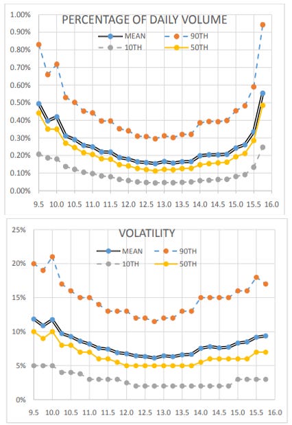
Notice the bottom of the U-shape showing the midday lull in volume and volatility.

I made a table characterizing the mean volume curve by hour. It’s not directly from the paper, but derived by eyeballing, but it’s perfectly adequate for our purposes.

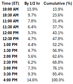
When I was a market-maker, our option models “decayed” the day in a similar pattern. There are 13 half-hour periods, but by 10am we believe more than 1/13 of the “vol time” had elapsed, yet from noon to 12:30 pm, the straddle barely decays. Our Option City streaming software let you specify a curve for how much time remained in the day for any hour.

Addressing the “overnight”

Another improvement to our assumptions is to acknowledge that the overnight period from 4 pm yesterday until 9:30am today, despite encompassing 17.5 out of 24 hours, does NOT represent nearly 2/3 of the market risk or volatility.

For exposition, we will show 2 different adjustments.

1) “Overnight has no volatility” assumption

This is naive in the opposite direction from the original calculations, which assumed that an overnight hour and a market hour were equal. In this adjustment, the straddle doesn’t start decaying until the market opens. The full decay occurs in just 6.5 hours.

2) “Overnight has 30% of the 24-hour volatility” assumption

We prorate the passage of time so that overnight DTE sums to .30 and the remaining .70 DTE is encompassed by trading hours.

Demonstration

This table assumes the U-shaped profile for how much volume has elapsed as a stand-in for how much time remains. The volume profile:

We construct pricing for both types of overnight assumptions.

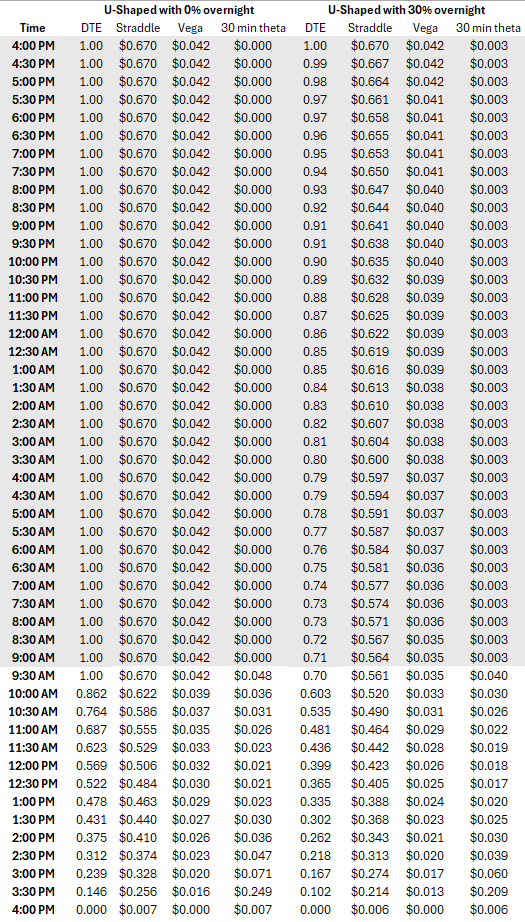
Visually:

In the naive 0% overnight schedule, the straddle doesn’t start decaying until the open and the decay is steeper intraday since there’s only 6.5 hours to erode the entire straddle.

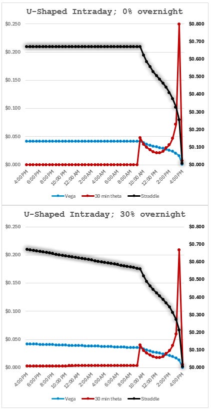
Let’s zoom in on the straddle trajectories because this highlights just how different one’s valuations can be as soon as the clock starts ticking and traders’ assumptions of DTE start diverging:

The straddles start and end in the same place but the interim is where the buys and sells happen.

Kevin’s 683 SPY call with 10 minutes until expiration

We’re going to roll with the compromise decay schedule since it’s the most realistic of the 3 choices:

U-shaped decay profile assuming overnight is 30% of the DTE

From the table, we see the last half-hour represents .102/365 DTE.

How about the last 10 minutes?

We could divide .102 by 3, but realistically (and the paper confirms this), the last 15 minutes contain even more “volatility time” than the second-to-last 15 minutes. Still, let’s be conservative and just divide by 3 since Kevin is buying.

DTE = .102/3
DTE = .034 

When Kevin bought the 683 call for $.02 he said SPY was $682.05 bid. Just to be thorough, let’s estimate the 682 straddle

SPY 10-minute straddle = .8Sσ√T
straddle = .8 x 682 x .16 x √(.034/365)
straddle = $.84

We are going to compute the call using a Black-Scholes calculator, but I like to inject homework questions when there’s an opportunity for estimation practice:

💡Estimate the 683-call based on the straddle price without an option calculator

I just used my Black-Scholes function in Excel with these inputs:

Stock price = 682.05
Strike price = 683
IV = .16
DTE = .034/365
RFR = 0

683 call = $.105

Those calls are realistically worth about a dime and Kevin lifted them for $.02!

Post-closes and contrary exercise

For Amercian-style exercise, expiration isn’t really 4pm because you can abandon an option that was in-the-money at 4pm or contrary exercise an option that was out-of-the-money.

This has a value. If suddenly there was a bomb dropped in the Middle East and USO expired just below the strike, you could exercise the calls to get long or abandon the slightly ITM puts. Similarly, if you were short the calls, you should expect to get assigned. If you were short the puts, you should expect not to get long at the strike as you will not be assigned.

Let’s say bearish news came out after the close while the futures are still trading. The futures tank. You can beta-weight all your prices from the close to construct a theoretical price for each name. Then make your contrary exercise and abandon decisions. You are effectively shorting the market at the closing price and then you buy the same dollar notional or beta-weighted notional in futures contracts to lock in a differential. You’ll have basis risk since your share positions won’t be in exact proportion with SP500 weights, but this will be small relative to your theoretical profit.

Likewise, if you are short options, you should expect to accumulate deltas in the wrong way, so you’d need to estimate how many wrong-way deltas you’ll acquire and hedge those with futures. While this will help have a neutral delta for the next day, you will have locked in a theoretical loss. Which makes sense — you were short options that turned out to have value after the close, so the 4pm mark did not reflect your actual p/l nor risk.

This matter of valuing options after the close is not academic. The procedure described here was a regular part of our expiration workflow and checks. This goes beyond equities too. In commodity options, there are “look-alike” European cash-settled versions of the American-style options. Since you can contrary an American style if the name was near pinning there would be an active market in the EOO or “exchange of option” which was the price for the euro-american “switch”. The American trades premium because you get another couple hours to look at the market so the switch was a referendum on the post-close straddle.

This was very common in natural gas options 15-20 years ago. EOOs didn’t trade electronically, so you basically had a mental scroll of where switches would tend to trade on past expiries to have an idea of what the post-close straddle could be worth. In practice, market-makers would always have the pins on the same way so they all needed to do the same risk-reducing trade, causing the switch to find a risk premium where a contra was content to either open or add more.

[I believe in 2018, the NYMEX changed American option specs so the options were auto-exercised at expiry. Probably to appease option shorts who didn’t like position surprises when they got their contrary assignment notices later in the evening.]

If you are long an equity option and your clearing firm doesn’t require you to decide to exercise/abandon until an hour after the close, (clearing firms have their own unique “cutoffs” and with a phone call you might be able to massage that) then you basically get a free look at the futures for the strikes near the expiry price.

Let’s say that hour could be worth as much as the mid-day 1-hour lull from 12:30-1:30pm or about .06 DTE. How would that have affected Kevin’s 683-call?

.06 + .034 (the DTE for the last 10 minutes of the day) = .094 DTE

The 683 call with .094/365 DTE is worth $.32 via B-S calculator or 3x what it was worth if you thought the post-close had no option value. In practice, the post-close is likely worth very little most of the time, and quite a bit in the event that news hits between 4 and 5pm.