
Options on Levered ETFs (part 2)
Last week, in part 1, we backfilled prerequisite knowledge:
- Distance in return space: equal percentage moves aren’t equal in compounded or log space
- Vol bonus vs vol tax: trend and chop change the distribution of a levered asset
- Derivatives-on-derivatives: options on the underlying ETF are inputs into pricing options on the levered ETF.
- Vega convexity: OTM options have “vol gamma” or volga which makes their sensitivity or vol changes vary depending on the IV level. This is not true for at-the-money (technically at-the-forward strikes) options.
Each of these ideas plays a role in the question that brings us here today.
How do we price options on a 2x levered ETF?
Besides being a practical question, especially with the explosion of levered ETFs hitting the market, this exercise in pricing options on levered ETFs offers something more valuable: it’s pedagogically isomorphic to the fundamental problem of pricing options in the first place.
Sorry for the big words: pedagogically isomorphic. But as I was working on this 2-parter, it conjured that familiar feeling that every derivatives trader would recognize — feeling your way through a problem that has an uneasy tension:
It feels like this should be a solved problem with an agreed-upon solution, but as you mentally step through scenarios, the path dependence suggests that it cannot be a solved problem.
To say that the pricing options on a levered ETF is isomorphic to pricing options in general is a recognition that the same essential structure repeats itself. In both cases, the solution depends critically on your assumptions, and the practitioner must understand how those assumptions bias the model’s output. The model doesn’t deliver a “true” price that you can mechanically apply. Instead, it invites discretion in interpreting its output, demanding that you recognize where your assumptions are doing the heavy lifting.
The bad news is that you won’t walk away from this post with an Answer with a capital A. The good news is there’s room for disagreement if assumptions vary which means there might be opportunity to trade.
Either way, I think the bridge between the concepts we backfilled earlier and how they affect option pricing on a levered ETF will not only be enlightening but tighten your grip on option concepts that feel slippery in application. You’re not just learning a technique; you’re developing judgment about when and how models guide decisions versus when they merely formalize your beliefs.
Starting Point: Double the Vol
We’ll start with the obvious observation: a 2x levered ETF has roughly twice the daily volatility of the unlevered one. That’s our baseline.
Imagine both ETFs trading at $100.
The unlevered ETF has an implied vol of 20% across all strikes.
A reasonable starting model is to double the volatility at each equivalent strike from the underlying.
But what counts as equivalent?
(In our example, we are saying all the strikes have the same vol, but in the real world where strike vols vary, this question of equivalent strike is critical.)
Percent vs Log Moneyness
If the unlevered ETF has a 90 strike (10% OTM), what’s the corresponding strike on the 2x ETF?
Under percent moneyness, the answer is 80. The formula for this:
Equivalent Strike For Percent Moneyness = 2K-S
For example: 90*2 - 100 = 80
A 10% move in the unlevered ETF means a 20% move in the 2x ETF.
But in log-space, the math gives you an 81 strike. We start with the definition of logdistance from Using Log Returns And Volatility To Normalize Strike Distances:
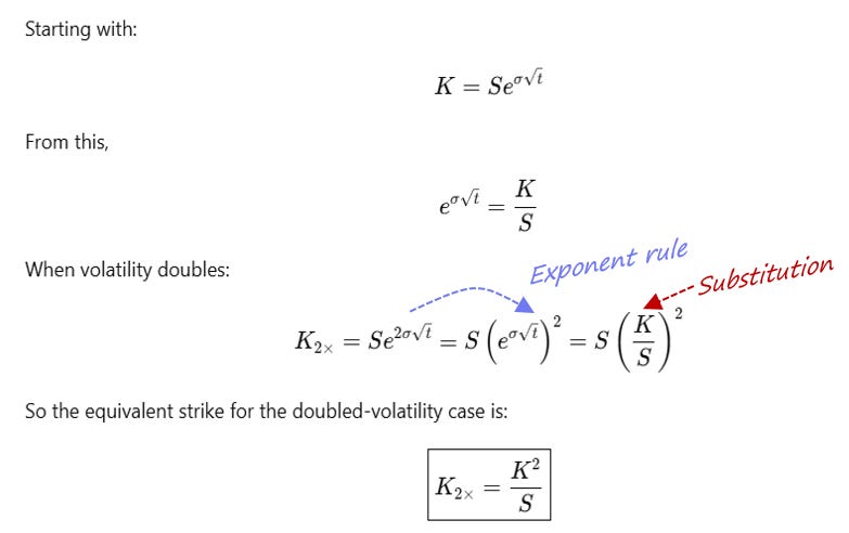
Equivalent Strike For Log Moneyness = K² / S
Both make sense—just not at the same time.
If the unlevered ETF gaps down 10% then the equivalent strike to the 90 strike will be the 80 strike for the levered ETF with 80 and 90 being the new ATM strikes, respectively.
But if the unlevered ETF meanders lower, accumulating a total return of -10% then the log return will have been slightly less. (Just think of how a 10% annual return must mean less than a 2.5% return compounded quarterly to get to the same place).
The point is that “equivalent strike” is an assumption, not a fact. Each definition carries a bias about how returns behave and we don’t know what held until after the fact.
For the sake of heuristics:
- Percent moneyness assumes fatter tails and linear compounding of shocks.
- Log moneyness assumes smoother diffusion and constant proportional risk.
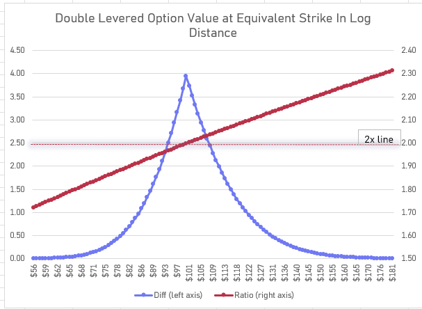
This table shows the equivalent strike and option values for the percent and log-monyeness assumptions:

Take note of the highlighted strikes which show how the difference in equivalent strikes vary as we get further from the spot price. Also note that distance when measured in standard devs for equivalent strike is the same for logmoneyness. This is a tautology as we defined distance in logspace or Black-Scholes terms.
💡The forward price
Another wrinkle in specifying the equivalent strike is the forward price. If the 2x ETF is hard-to-borrow but the regular ETF is not, the ratio of forward prices will be different than the ratio of the spot prices. The equivalent strike by any method will end up accounting for that if you replace S with F in the formulas. But if you have a pair vol trade on between the unlevered and levered ETF you are also exposed to any changes in the funding differentials between the 2 names because it will be inherited by the option prices.
Observing the effect on OTM calls vs OTM puts
If we price the 2x ETF’s options using log-equivalent strikes and double vol, the ATM options will indeed be about twice as expensive as their unlevered counterparts.
OTM strikes won’t scale that cleanly.
OTM calls on the levered ETF will be worth more than 2x at the equivalent strike while OTM puts will be worth less than 2x.
You can likely explain this in several ways. For our purposes, which ultimately is about pricing options, our going to attribute this phenomenon to volga aka “vol gamma.”
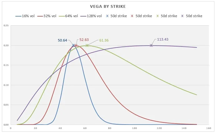
In Finding Vol Convexity, you see a chart of vega at different vol levels. You can infer that OTM call volgas are higher than OTM put vegas as they are “picking up more vega” as vol increases.
💡A non-visual explanation
We can reason our way to the same conclusion by recalling arbitrage bounds. Upside call values are arbitrage bounded by the stock price which itself is unbounded. Put max values on the other hand are bounded by the strike price. Upside options have more to gain from vol going up.
The Problem with Doubing Vol: Amplifying Skew
While doubling vol doubles the value of ATM options, it more than doubles OTM options because vol convexity makes them increasingly sensitive as IV rises.
Recall this chart from part 1:
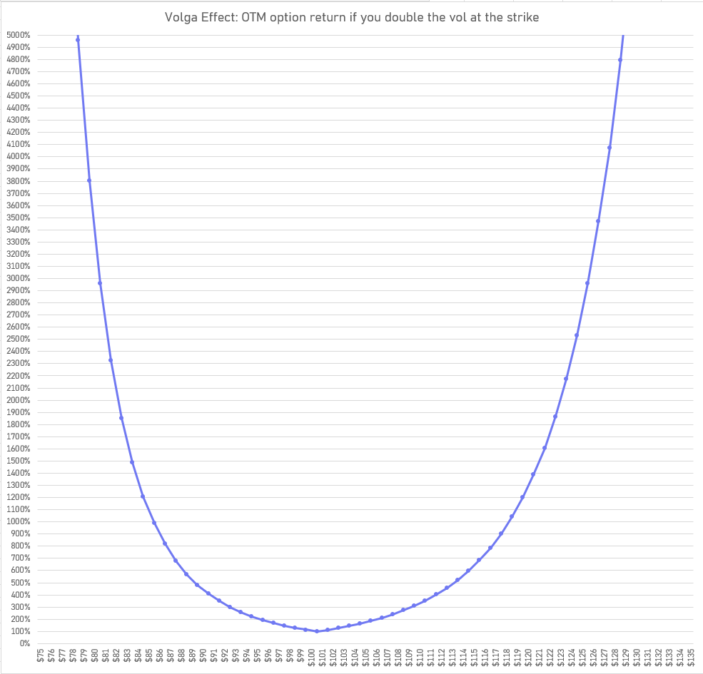
What’s the problem? Doubling vol, especially on already skewed puts, risks modeling put spreads too cheap.
To keep vertical spreads from becoming unrealistically cheap, the levered ETF’s vol surface likely has flatter skew than the underlying’s—it passes through less of the amplification than a pure 2x model would predict.
🧪An untested hypothesis
As an example of something I might try to throw against the wall:
Perhaps the lower strike put shouldn’t trade below the price that keeps an equidistant, vega-neutral put spread identical between the levered and unlevered ETFs.Sometimes model-building is oberving the market prices, trying to fit the behavior, and then trying to reverse-engineer what rule, in words, the streamer’s model seems to be projecting.
The Problem with Return Assumptions: Path Dependence and Time Resolution
In Risk Depends on the Resolution, I show that volatility scales not only with sampling period* but with time.
💡The coastline paradox
This is not just a property of vol. The length of a coastline is not a given. It depends on the length of ruler you use to measure it.
A 6σ daily move is possible. (It happened on Oct 10th intraday in IWM)
A 6σ annual move is a fantasy.
As explained earlier, the “correct” equivalent strike depends on how you assume vol scales with time. Black-Scholes’ lognormality says variance is linear with respect to time (or volatility is proportional to root time). It’s just an assumption.
Realistically, equivalent-strike mapping probably has a curved relationship with time, with the growth process looking more lognormal as you go out in maturity.
Reconciling the Trade-offs
Skew amplification
We have competing effects:
Fat tails, especially in near-dated or same-day maturities, demand higher vols, but that same adjustment can make longer-dated put spreads too cheap.
The skew might vary in the unlevered ETF to account for the time-dependence of distributions, but the effect is amplified when we double the vols. The pass-through values risk being excessive.
My guess:
Levered ETFs should show larger vol premiums than 2x for the far OTM put tails (1-5d deltas) in near-dated expiries but smaller than 2x differences in vols at equivalent strikes for meatier strikes (say 5-30d).
🧪Testable expression of this idea: Is the 45/25/5 delta put fly empirically expensive if you used 2x vol at equivalent strikes?
Browsing option surfaces, skewed options at equivalent strikes on SSO and NVDL (2x versions of SPX or NVDA) trade at lower vols than 2x the underlying ETF vols just based on 1-5 month expiries.
Market widths mask what’s going on in the far tails of the 2x ETFs or in some cases the strike ranges don’t go far enough.
Path dependence and modeling the stock process
You can always try pricing options on the 2x by Monte Carlo simulation based on a tree of the underlying.
You still need to specify a diffusion process. Just a thought on that:
My former colleague at SIG, quant Vivek Rao, has a repo that simulates terminal prices (not log prices) under a Student-t process and makes the case that this conforms better to the vol smiles we actually see in markets. This might be especially relevant for nearer-dated distributions, which look more normal than lognormal.
Wrapping up
No matter how you price options on a 2x ETF there will be a bias. Even the simple question of which strike on the levered ETF maps to the unlevered ETF depends on assumptions of the stock diffusion process.
If you use percent difference (ie 2K-S) you will structurally underprice the 144% call versus some using log difference (K² / S) to find the equivalent strike. The path (trend vs chop) will ultimately be the judge of who was right.
I suspect this is how I got smoked to a short SCO (inverse levered oil) call back in 2014 after OPEC lifted production quotas to bury the US shale competition. Oil went down relentlessly in a crescendo of fundamental realignment and self-reinforcing gamma flows as oil liquidity providers are structurally short puts. A seemingly far OTM SCO call turned out to be “much closer” because of the path USO took.
(Think of it this way: if USO goes down 10% 2 days in a row, the stock is down cumulatively 19%. The inverse levered ETF is up 44% not 38%).
These modeling problems are endemic to option pricing, generally not just levered ETFs. If you price options by sampling vol daily instead of weekly in a name that trends, you’ll sell the option too cheap. The problem is that you extrapolated vol via root time but that understates vol for a trending asset.
[See Adjusting volatility for autocorrelation. If only we knew ahead of time if an asset would trend or mean-revert!]
Pricing options forces you to stare straight at your assumptions. The path, the volatility resolution, the return process—all of it shapes how “equivalence” behaves.
The point isn’t to fix the bias but to know which way it leans. This awareness is the space between what’s priced in and how it differs from your analysis. It’s the foundation of disagreement and ultimately trades.