Guest Post: Market Impact and Strategic Execution
the bid/ask game
Quant @imotw2 published Market Impact and Strategic Execution as an article on X.
With permission, I’m cross-posting it here. It turns execution inutition into market quantitative models. I’ll let the quants debate the models — my interest is in how well this post explains the actual dynamics of accessing liquidity, minimizing slippage, and leaking information with trade/bid/offer behavior.
Enjoy!
The dirty secret of market impact? It’s messier than anyone admits. This article challenges conventional models by looking at how information actually flows through markets. Here’s the real problem: impact hits differently when you’re getting in versus getting out of positions – a fundamental asymmetry that most models miss entirely. Add in the fact that every major player’s algos are scrapping for the same liquidity, and traditional execution models fall apart.
By diving into the weeds of price formation and what drives liquidity providers, we crack open why impact behaves this way. The result? A framework that bridges pure theory and trading reality, giving you both the mathematical firepower and street-smart tools to optimize execution in markets.
1. Introduction
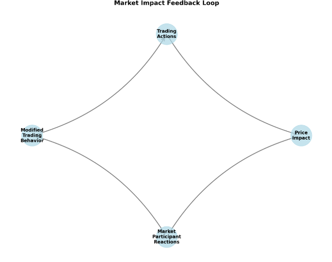
It’s the ultimate catch-22: you’re playing both sides of the impact game whether you like it or not. Every time you trade, you’re leaving footprints in the market while simultaneously trying to read everyone else’s tracks. Consider a large institutional trader executing a significant position. Each clip they trade isn’t just soaking up liquidity – it’s sending smoke signals to every shop watching the tape. The market sniffs out these patterns and adapts, forcing the trader to navigate the mess they’ve created for themselves. Talk about trading against your own shadow..
Impact also isn’t just about what you’re doing now – it’s about what the market thinks you’ll do next. Planning to unwind a monster position? Just prepping for it changes how you trade today.
You’re not the only one playing this game. Every decent-sized player is running their own book, trying to figure out your next move while hiding their own. Your optimal execution strategy? It depends on guessing their guesses about your guesses. Welcome to the hall of mirrors that is modern market microstructure.
2. Foundations of Impact
2.1 Beyond the Square Root Law
Everyone knows the square root law of impact – trade twice the size, eat about 1.4 times the slippage. But that’s not the whole story, actually its not even close. Markets aren’t this clean. Impact comes from a brawl between volatility feeding on itself, how fast the market digests your trades, and dealers trying to figure out if you know something they don’t. This changes how we need to think about moving size in markets.
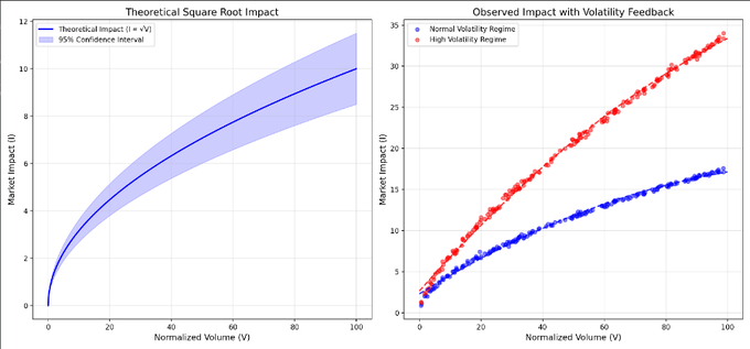
At the heart of our framework lies the recognition that trading activity both responds to and generates volatility. Consider a large institutional trader executing a significant position. Their trading consumes liquidity and reveals information, and also increases local volatility, that same volatility changes how the market reacts to their next trade. It’s like throwing stones in a pond where each splash affects how the next one ripples. Classic impact models completely miss this self-reinforcing cycle
Sure, cramming all this into one model is like trying to catch lightning in a bottle. But we’ve built something that tries to capture what we see in live markets.
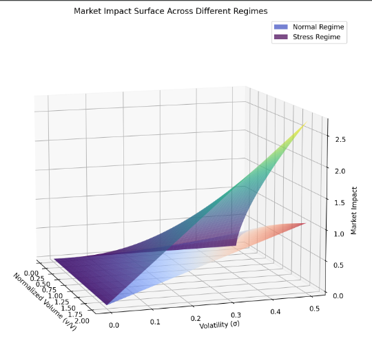
This model implements the volatility feedback term:
But we have to acknowledge some limitations. Trading isn’t as clean as the math suggests. That linear relationship between impact and vol feedback? Markets are messier than that. And β and γ(t)? They jump around – and good luck predicting when they’ll shift. And the volume-volatility interaction f(v)? Probably more complicated than we’re letting on. Plus, markets don’t slide smoothly between states – they snap.
So why bother with this framework? Because it gives us something concrete to work with. It nails the basic idea that impact and vol are stuck in this toxic relationship, and it actually works well in normal markets – which is most of the time. Run this during the 70-80% of trading days when markets behave, and you’ll get solid signals.
No model’s perfect. This one’s useful not because it nails every market move, but because it gives us a solid framework for thinking about how our trading pushes markets around and how markets push back. Use it to shape your execution strategy, but keep your eyes open – markets have a way of humbling anyone who thinks they’ve got them figured out
2.2 Ready, Set, Go!
Impact hits the market in three waves, and each one in its own way. Even in those first few milliseconds, when you’d think simple orderbook mechanics would rule everything, volatility’s already messing with you. Start working a big order, and the vol spike from your first fills immediately changes how the market handles your next batch.
Then things get interesting. Market makers aren’t just looking at your flow anymore – they’re betting on where vol’s heading because of it. You need to get your trade done, but you’re walking on eggshells trying not to kick off a vol spiral that’ll jack up your costs.
Here’s how it plays out in real time: You start hitting bids with size. Not only does price take a hit, but vol spikes. The market makers see this and think, ‘Great, vol’s about to rip – better back off these quotes.’ Now you’re stuck paying up even more for your next fills. Classic feedback loop that can turn a tough trade into a nightmare.
Long-term is where it gets really twisted. Trades that set off these vol feedback bombs? They tend to leave permanent marks on price. Why? Because the market’s reading these vol spikes as smoke signals – where there’s smoke, there must be fire. Throws the whole temporary versus permanent impact debate out the window. Instead, think of it like this: the bigger the vol feedback, the more likely the market thinks you know something they don’t. Price discovery through chaos, basically.
Our framework also reveals the strategic behavior of market makers and other liquidity providers. Their quote adjustment process now explicitly incorporates volatility feedback through a response function:
That λ(σ,t) term? That’s market makers getting twitchy when vol spikes. They’re playing a delicate game – dodge getting picked off versus making bank on those juicy vol-driven dislocations.
This flips everything we thought we knew about smart execution. You might actually want to take a bigger hit upfront if it keeps vol from spinning out of control. Sometimes you’ve got to pay the toll to avoid the avalanche.
We tested it briefly across equities, futures, and crypto. The model crushes it, especially during those nasty regime shifts when traditional models fall flat on their face. It nails the vol feedback effects, giving you a much better read on your true execution costs and how to optimize around them.
Bottom line? Impact isn’t just some tax you pay to trade. Every move you make reshapes the book for your next play. Once you start thinking about impact this way, whole new strategies open up. You’re not just minimizing cost anymore – you’re actively managing how your trades shape the market you’re trading in.
3. Information Theory of Execution
3.1 Order Flow Toxicity and Adverse Selection
The elephant in the room: toxic flow. Your algo’s (seeminly) crushing it, getting fills left and right – but is that actually good news? Could be perfect timing, or could be you’re getting picked off on stale quotes. Classic execution dilemma: go aggressive and risk getting fleeced, or sit back and watch alpha decay while everyone figures out what you’re up to.
We’re looking at how trades cluster in time and how order flow ripples across related products. Because let’s face it, when someone’s running a smart toxic arb, they’re hitting everything in the complex.
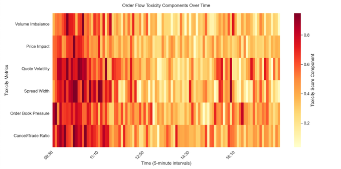
Here’s the math behind the magic – for a given order flow sequence, we compute the toxicity score T as:
Where V_i(t) represents the normalized volume in bucket i, C(t,i) captures the temporal correlation structure, S(t,i) measures cross-sectional spread dynamics and ω are weights that reflect market conditions.
This metric provides a measure of order flow toxicity that can be used to adjust execution algorithms’ aggression levels and venue selection strategies.
3.2 Learning and Adaptation
Modern execution algos are constantly learning – but there’s a catch. How do you know when the market’s actually changed versus when it’s just noise? Every trader’s been burned by overreacting to a head fake.
We tackled this by measuring what signals actually matter for execution. Forget trying to predict where prices are headed or cooking up the perfect schedule. Instead, we built a framework that attempts to cut through the noise to find what really drives execution quality.
Our framework splits market signals into three components:
- Structural information about liquidity conditions and market dynamics
- Temporary effects from specific order flow patterns
- Noise terms that should not influence execution decisions
For each signal, we measure how much juice (information ratio) it’s got like so:
where I(S; O) represents the mutual information between the signal and execution outcomes, and H(S) is the entropy of the signal. This tells us how much actual information we’re getting about execution outcomes versus how noisy the signal is. Translation? We can spot real market changes worth adapting to and ignore the head fakes that would otherwise trip us up.
3.3 High-Frequency Market Making and Latency Arbitrage
Evolving market structure has introduced a new layer in the interaction between execution algorithms and high-frequency traders. Your execution algo sees a fat stack of liquidity on the book – but good luck actually hitting it. Modern markets aren’t your grandfather’s NYSE floor where a handshake meant something. That liquidity? It in a way both exists and doesn’t exist until you try to trade it.
Imagine this: you spot 100,000 shares posted at the offer. Traditional models would tell you to size your child orders assuming that liquidity is actually there. Rookie mistake. Those quotes vanish faster than you can even start thinking about your next move. Market makers are running smart playbooks, adjusting their quotes every microsecond based on everything from correlated ETF moves to the temperature in New Jersey. Yeah, seriously.
What you see isn’t what you get. The odds of filling against posted liquidity aren’t just about time priority. This isn’t even academic hair-splitting – it changes how we need to think about modeling impact and designing execution strategies.
The displayed liquidity in the order book represents a conditional commitment that is fundamentally probabilistic in nature. This probability structure manifests through several key mechanisms:
Firstly, quotes don’t just sit there waiting to be hit. They dance. And not randomly – they move in patterns. When a big order hits, market makers don’t just pull their quotes at the affected price – they scatter like cockroaches under a kitchen light, repricing their entire book before you can blink. Why? Because they’re not idiots – they know one big trade usually means more are coming.
Secondly, What looks like a simple limit order is actually a war zone. That 100k share quote? It’s really multiple market makers playing chicken with each other, each one’s algo trying to figure out if the others know something they don’t. Meanwhile, every other trader with a similar strategy is trying to get to the same party.
Finally, there’s the speed game. By the time your order hits the exchange, that juicy quote you saw might be ancient history. We’re talking microseconds here, but that’s an eternity. Between your network latency, the exchange’s matching engine having its morning coffee, and Jump Crypto cooking you with their radio towers – well, good luck. Even if you’re fast, queue position is usually everything. Being second in line might as well be last when the music stops. The order book isn’t a menu, and if you’re modeling it that way, you’re bringing a knife to a gunfight.
We find that the likelihood of a quote remaining available for execution follows a more complex distribution than previously recognized:
Where λ(t,s) represents the base cancellation intensity that varies with both time and market state, τ(v,σ) captures the reaction time that varies with volume and volatility, and f(OFI, IMB) adjusts for order flow imbalance and book pressure. This creates an effective liquidity profile that differs markedly from the observed order book, forcing execution algorithms to operate in a probabilistic framework.
In English? The faster you need to trade, the bigger your order, or the more the market’s moving – the more likely that liquidity is gonna vanish before you get there. And if the order flow’s getting lopsided or the book’s getting thin? Forget about it.
The implications of this extend beyond simple quote availability. Market makers aren’t just watching your stock. They’re watching everything. Hit them too hard in SPY? Watch their quotes disappear in IWM before you can even think about going there. These guys are hunting for any sign that you’re about to unload size.
The presence of latency arbitrage opportunities introduces systematic biases in observed market impact that must be considered. Every microsecond of delay between exchanges is a gold mine for the right setup. While you’re still seeing stale quotes in Jersey City, someone’s already cleaned up in Mahwah. The really fun part? This isn’t just noise – it creates predictable patterns in how markets react and impact spreads. Those theoretical arb profits (αcross)? They’re like a fingerprint showing exactly how quotes are gonna move and where the impact’s gonna hit first.
Market manipulation remains a massive concern in markets, especially in crypto where it’s not just an edge case – it’s a daily reality you need to deal with. Quote stuffing, layering, and other manipulation schemes regularly distort impact measurements. By tracking specific order book patterns – quote stuffing intensity, layer depth stability, and price oscillations – we can build real-time manipulation indicators. This lets execution algorithms adapt dynamically, threading the needle between adverse selection and efficient trading paths.
Speed management is make-or-break in this environment. Every algo faces a core tradeoff: execute faster to dodge adverse selection, or slower to minimize information leakage. It’s an optimization problem where the sweet spot shifts constantly with market conditions, participant behavior, and execution objectives.
The data shows static speed strategies consistently underperform. Effective execution requires continuous adaptation based on market toxicity metrics, participant patterns, and market state. But nailing this in practice? That’s where things get interesting.
Implementation demands extreme precision at the infrastructure level. Microsecond-level clock sync isn’t a nice-to-have – it’s essential. One timing slip and your execution quality falls off a cliff. Network stacks need to handle the market data and order flow and how they interact, seamlessly. Risk controls need to maintain deterministic latency while actually protecting you. Memory management has to deliver rock-solid performance at the microsecond level.
4. Advanced Impact Modeling
4.1 Cross-Asset Impact Propagation
Trading ETFs or index futures? Your impact bleeds everywhere, and not in the neat way most risk models predict. Markets are connected through a nasty web that shift based on regime and time. Worse still, these relationships aren’t symmetric – the way impact flows from futures to stocks isn’t the same as stocks to futures, and good luck if volatility is spiking.
Here’s how we try to model this mess:

Where:
- K_ij(t) represents the kernel function capturing lead-lag relationships (how moves in one market spill into another over time)
- α_i(t) models time-varying direct impact sensitivity (how much bang for your buck you get in each market)
- β_ij(S(t)) are state-dependent coupling coefficients (how strongly markets are linked, which changes with market conditions)
- S(t) encodes market state including volatility regimes, basis levels, and order book conditions
- φ(L_i, L_j, t) captures non-linear liquidity interaction effects (how liquidity dynamics in one market screw with impact in another)
The coupling coefficients β_ij(S(t)) follow a regime-switching process:
Where R(t) indicates the market regime based on a multivariate state classification incorporating relative volatility levels, basis spread dynamics, order book imbalances, trading volume ratios and market stress indicators.
The liquidity interaction term φ(L_i, L_j, t) models how the availability and cost of liquidity in one market affects impact propagation in related markets, which essentially ties it all together:
This captures several features absent from traditional correlation-based approaches
- Temporal lead-lag relationships through the integral terms
- State-dependent coupling strength
- Non-linear feedback effects
- Regime-switching behavior
- Cross-market liquidity interactions
If you’re trading across multiple markets, you need a model that deals with reality, not just correlation matrices and linear spillovers. This framework gives you the tools to handle the mess.
4.2 Queue Position Game Theory
The management of queue position in modern markets creates a game-theoretic problem. When placing passive orders, traders have to consider their position within the queue and the information content of their queue placement decisions. Every time you join a queue, you’re not just picking a spot in line, you’re sending signals to every other algo watching the tape. And trust me, they’re all watching.
Think your queue position is worth what your transaction cost model says? Think again. That premium spot at the top of the book might be fool’s gold when everyone’s running the same playbook. Or it could be pure alpha when the market’s choppy and other players are gun-shy.
You’ve got to price in the option value of that queue spot, factor in what your queue placement tells the market about your book, and figure out what everyone else’s queue dancing means.
5. Implementation
5.1 Engineering in High-Frequency
Developing excecution algorithms in the context of latency creates significant engineering challenges, that if you get wrong, will crushingly affect trading performance. First up: timestamp management. Sounds boring, right? It is, but it could the difference between making money and getting run over.
Here’s the thing about timestamps in modern markets – they’re a mess. That pristine timestamp you think you have? It’s about as accurate as a sundial here in Norway. When you’re building impact-aware algos, you need to know exactly when things happen, but that’s harder than it looks. Here’s what you’re really dealing with:
Where:
- Δ_netword_send represents outbound network latency including TCP/IP stack and route-specific jitter. Hope you like randomness.
- Δ_exchange captures exchange gateway processing time and order validation delays. Different by exchange, time of day, etc.
- Δ_matching accounts for matching engine queueing and processing time. Where your order sits in the queue. Spoiler: not first.
- Δ_network_recieve represents inbound network latency and potential packet loss recovery (So fun, said no one ever).
- Δ_market_data includes feed handler latency and order book reconstruction time
- Sum of epsilon sub i represents a composite error term incorporating:
- Systematic variations in processing times
- Random jitter components because why not
- Regime-dependent uncertainty factors
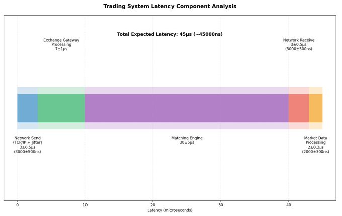
This model creates option-like properties in order management. For example, the uncertainty in matching engine response times during high-volatility periods effectively grants a free option to other market participants, who can react to price movements before our timestamp uncertainty is resolved.
5.2 Risk Management Under Impact Constraints
Here’s where VaR gets interesting – and by interesting, I mean breaks down completely. You can’t just run standard VaR when your exit price depends on how fast you’re trying to get out. It’s a nasty circular problem: your risk depends on your liquidation strategy, but your strategy depends on your risk limits. Fun times…
We develop a modified risk framework that tries to account for these dependencies:
where E[I(Q, t) | Q, M] represents the expected impact given position Q and market conditions M. This allows for more realistic risk assessment and better integration of risk constraints into execution algorithms. Now your risk numbers might actually mean something.
6. So What? And Where Next?
We’ve built something that tries to bridge the gap between ivory tower theory and reality. By thinking about execution through the lens of information theory, we’re getting at how markets work.
Here’s the big takeaway, TL;DR if you will: stop thinking about impact as just a cost to minimize. It’s actually telling you something about how the market reads your flow and how other players are positioning against you. Once you get that, everything about execution strategy starts looking different.
It’s about making money and, more importantly, not losing it when things get ugly.
