Geometric vs Arithmetic Mean In The Wild

Review

In ‘Well What Did You Expect’? we learned:

• Mathematical “expectation” is a simple average or arithmetic mean of various outcomes weighted by their probability
• Arithmetic means are familiar. Your average score in a class is the sum of your test scores divided by the number of tests. If you score 85, 90, 98  your average for the class is:  (85+90+98)/3 = 91
  
  Note the scores are weighted equally.
  
  Here’s what the number sentence looks like without factoring out the 1/3:.33 * 85+ .33 * 90 + .33 * 98 = 91
  
  If the final test is worth 50% of the total grade the weighted average is computed: .25 * 85 + .25 * 90 + .50 * 98  = 92.75
  
  Whether we are weighting the results equally or not, we are still computing the average by summing, then dividing.
  
  Geometric means are like arithmetic means except quantities are multiplied instead of summed. Since investing is the process of earning a return and reinvesting the total proceeds we are multiplying, not summing results. If you invest $100 at 10% for 5 years your final wealth is given by:
  
  $100 * (1.10) * (1.10) * (1.10) * (1.10) * (1.10)  or simply $100 * (1.10)⁵ = $161.05
  
  In life, we often know the ending amount and the initial investment but want to know “what was my average growth rate per year?”
  
  The answer to that question is not the simple arithmetic average but the geometric average because we were re-investing or multiplying our capital each year by some rate. That rate is known as the CAGR or “compound annual growth rate”.
  
  If we start with $100 and have $161.05 after 5 years we compute the geometric average in an analogous way to arithmetic averages, but instead of dividing by the number of years, we take Nth root of our total growth where N is the number of years we compounded for.
  
  CAGR for 5 years = ($161.05/$100) ^ (1/5) -1 = 10% [we subtract that 1 at the end to remove our starting capital and just have the rate]

CAGR vs Simple Average Returns

With investing we are almost always re-investing our capital. That means our capital is being multiplied by a rate from one period to the next. When we want to know the average rate, we really want to pick the geometric average not the arithmetic one (there are other types of averages too like the harmonic average!). We want to compute the CAGR.

As a last proof that the CAGR and simple arithmetic average are different we can revisit the example above. If we compound an initial capital of $100 at 10% per year for 5 years we end up with $161.05 for a total return of 61.05%.

If we compute the simple average:

61.05% / 5 = 12.2%

This is higher than the CAGR of 10%

This is a consistent result. The geometric mean is always lower than the arithmetic mean!

How much lower?

It depends on how volatile the investment is. The reason is intuitive.

Imagine making 50% and losing 50%. The order doesn’t matter. You have net lost 25% of your initial capital.

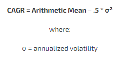
The formula that relates the arithmetic mean and CAGR:

This Is Not Just Theoretical

I grabbed SP500 total returns by year going from 1926-2023. Here’s what you find:

Simple arithmetic mean of the list: 12.01%

Standard deviation of returns: 19.8%

These are actual sample stats.

What did an investor experience?

If you start with $100 and let it compound over those 97 years, you end up with $1,151,937. 

What’s the CAGR?

CAGR = ($1,151,937 / $100)^(1/97) – 1 

CAGR = 10.12%

These are the actual historical results. An average annual return of 12.01% translated to an investor’s lived experience of compounding their wealth at 10.12% per year. 

Comparing the sample to theory

If you knew in advance that the stock market would increase 12.01% per year and you used the CAGR formula with our sample arithmetic mean return and standard deviation, what compound annual growth rate would you predict?

CAGR = Arithmetic Mean – .5 * σ²

CAGR = 12.01% – .5 * 19.8%²

CAGR = 10.06%

An average arithmetic return of 12.01% at 19.8% vol predicted a CAGR of 10.06% vs an actual result of 10.12%

Not too shabby. 

I used the same parameters to run a simulation where every year you draw a return from a normal distribution with mean 12% and standard deviation of 19.8% and compounded for 97 years.  

I ran it 10,000 times. (Github code — it works but you’ll go blind)

Theoretical expectations

CAGR = median return = mean return – .5 * σ²

CAGR = .12 – .5 * .198² = 10.04% 

Median terminal wealth = 100 * (1+ CAGR)^ (N years)

Median terminal wealth = $100 * (1+ .104)^ (97) = $1,072,333

Arithmetic mean wealth = 100 * (1+ mean return)^ (N years)

Arithmetic mean wealth = $100 * (1+ .12)^ (97) = $5,944,950

The sample results from 10,000 sims

The median sample CAGR: 10.19%

The median sample terminal wealth = $1,2255,90

The mean terminal wealth: $5,952,373

Summary Table

The most salient observation:

The median terminal wealth, the result of compounding, is much less than what simple returns suggest. When you are presented with an opportunity to invest in something with an IRR or expected return of X, your actual return if you keep re-investing will be lower than if you take the simple average of the annual returns.

If the investment is highly volatile…it will be much lower. 

The distribution of terminal wealth

The nice thing about simulating this process 10,000x is we can see the wealth distribution not just the mean and median outcomes.

Remember the assumptions:

• Drawing a random sample from a normal distribution with a mean of 12% and standard deviation of 19.8%
• Assume we fully re-invest our returns for 97 years

And our results:

• The median sample CAGR: 10.19%
• The median sample terminal wealth = $1,2255,90
• The mean terminal wealth: $5,952,373

This was the percentile distribution of terminal wealth:

The mean wealth outcome is 5x the median wealth outcome due to a 2% gap between the arithmetic and geometric returns. The geometric return compounded corresponds exactly to the median terminal wealth which is why we use CAGR, a measure that includes the punishing effect of volatility. 

In terms of mathematical expectation, if you lived 10,000 lives, on average your terminal wealth would be nearly $6mm but in the one life you live, the odds of that happening are less than 20%.

The chart was calculated from this table:

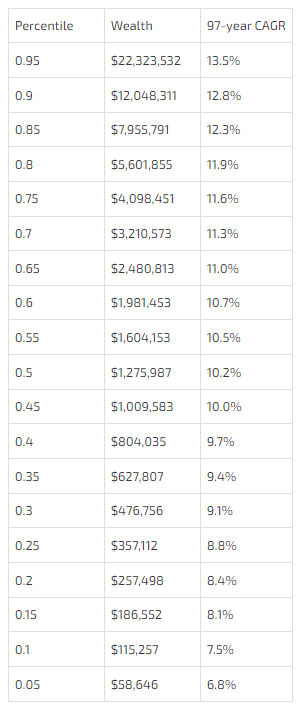
Note that, also 20% of the time, your $100 compounded for 97 years turns into $257,498 or a CAGR of 8.4%. A result that is 1/5 of the median and 1/20 of the mean. Ouch. 

So when someone says the stock market returns 10% per year because they looked at the average return in the past, realize that after adjusting for volatility and the fact that you will be re-investing your proceeds (a multiplicative process), you should expect something closer to 8% per year. 

And one last thing…you should be able to see how rates of return, when compounded for long periods of time, lead to dramatic differences in wealth. Taxes and fees are percentages of returns or invested assets. Make sure you are spending them on things you can’t get for free (like beta).

A Question I Wonder About

If you draw a return a simple return at random from a normal (ie bell curve) distribution and compound it over time, the resultant wealth distribution will be lognormally distributed with the center of mass corresponding to the CAGR return.

We saw that theory, simulation and reality all agreed. 

Or did they?

The simulation and theory were mechanically tied. I drew a random return from N [μ=12%, σ = 19.8%] and compounded it. But reality also agreed.

It may have been a coincidence. Let me explain. 

Stock market returns are not normally distributed. They are well-understood to differ from normal because they have a heavy fat-left tail and negative skew.

1. The fat-left tail describes the tendency for returns to exhibit extreme (ie multi-standard deviation) moves more frequently than the volatility would suggest.
2. Negative skew means that large moves are biased toward the downside.

These scary qualities are counterbalanced by the fact that the stock market goes up more often than it goes down. In the 97-year history I used to compute the stats, positive years outnumbered negative years 71-26 or nearly 3-1. 

The average returns, whichever average you care to look at, is the result of this tug-of-war between scary qualities and a bias toward heads. With the distribution not being a normal bell curve it feels suspicious that the relationship between CAGR and arithmetic mean returns conformed so closely to theory.

I have some intuitions about negative skew (that’s a long overdue post sitting in my drafts that I need to get to) that tell me that in the presence of lots of negative skew, volatility understates risk in a way that would artificially and optically narrow the gap between CAGR and mean return. By extension, I would expect that the measured CAGR of the last 97 years would have been lower relative to the theory’s prediction. 

But we did not see that.

I have 2 ideas why the CAGR was held up as expected, despite non-normal features that should penalize CAGR relative to mean return. 

1. Path
   In Path: How Compounding Alters Return Distributions, we saw that trending markets actually reduce the volatility tax that causes CAGRs to lag arithmetic returns. It’s the “choppy” market that goes up and down by the same percent that leaves you worse off for letting your capital compound instead of rebalancing back to your original position size. The volatility tax or “variance drain” occurs when the chop happens more than trends (holding volatility constant of course). But since the stock market has gone up nearly 3x as often as it went down perhaps this trend compounding “bonus” offset the punitive negative skew effect on CAGR. 
   

What negative skew?

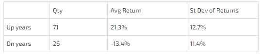
Using annual point-to-point returns, I’m not seeing negative skew. 

I’ve exhausted my bandwidth for this topic so I’ll leave it to the hive. Hit me up with your guesses.