embedding spot-vol correlation in option deltas

Before we get to the heart of today’s education, this is a video follow up to yesterday’s HOOD: A Case Study in “Renting the Straddle”.

I talk about oil volatility as well and how it shows up in the Trade Ideas tool.

This concept of “spot-vol correlation” gets a lot of airtime from different angles even when it’s not explicit. The mass financial media doesn’t use the exact words but they know enough to call the VIX the “fear gauge”. VIX is a complicated formula that aggregates values representing annualized standard deviations from a strip of inverted Black-Scholes numerical searches with quadratic weights. But all of this gets translated to:

“when stock go down, that number go up”

That travels a lot faster. Even your cat knows that market volatility has an inverse relationship with stock returns.

The more your paycheck depends on option greeks, the more you will need to zoom in on this concept. Mostly because the relationship between vol and prices changes your actual risk. The Black-Scholes world assumes vol is constant, but we know better. The sensitivity of options to various market inputs (greeks are measures of risk) is naive without adjusting for behavior that is predictable enough for your cat make a better guess than random about what will happen to vol when stocks move.

How can use this cat knowledge to estimate better deltas so when our model says we are long $50mm worth of SPY, we aren’t suprised when it seems to act like we are only long $40mm worth?

There isn’t a single way to do this but I’m going to show you how I did it as a calculus-challenged orangutan.

Before we get to numbers and pictures, I want to mention one last thing.

There’s a riddle in the world’s best trading book Financial Hacking. An imaginary bank trader calls a meeting with management and says he’s found “greatest trade in the world”. He sits them down for a presentation and says he can buy calls for 20 vol and sell puts at 40 vol, delta hedge until expiry, and make a 20 point “arb”.

What’s the problem?

There are several, perhaps many, option traders reading this right now who have thought about the holy grail of long gamma, collecting theta. Look you can go do this right now.

1. Sell a strangle on 1-month oil futures and buy a ratio’d amount of 12-month CL straddles.
2. Buy a ratio time spread in a name that has a major event coming up
3. Trade SPY risk reversals

All of these trades will give you the “desired greeks”. But these are illusions. In order:

1. The lower vol on the deferred future makes the gamma of those options look higher than it is, but you need to weight the gamma by the lower beta those futures have to spot oil prices
2. The decay you think you collect on the near-dated short is unadjusted for the “shadow theta” or glide path of IV increasing as the upcoming event is a greater proportion of the variance remaining as each second elapses
3. Spot-vol correlation means that theta number is not just the cost of gamma but vanna. The owner of the put is getting more than gamma.

Ok, time for less words and more F9.

I grabbed a SPY IV curve from earlier this week. 31 DTE.

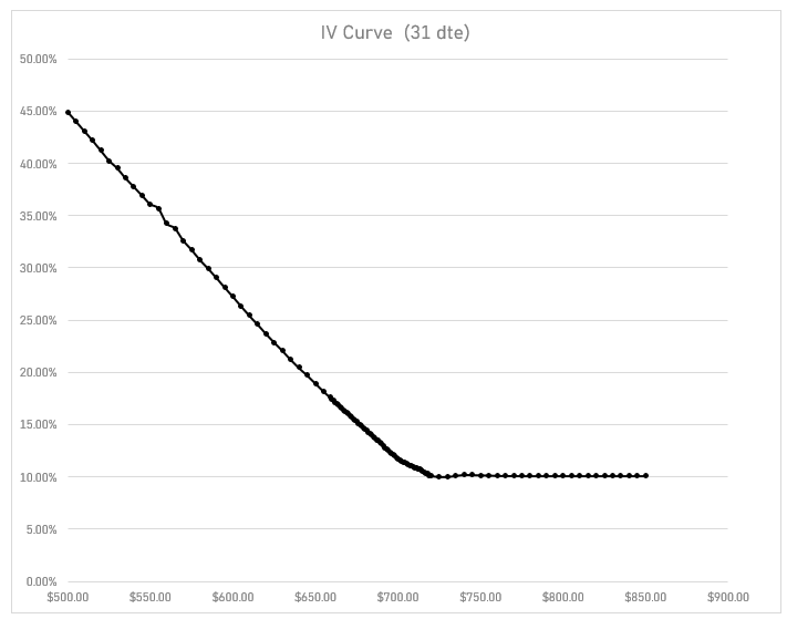
The spot price was $695.27 at the snapshot time but we are just going to keep things simple by ignoring any cost of carry and saying that spot is $695. I just wanted a sensible IV curve for demonstration purposes.

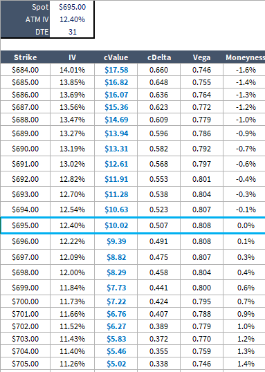
The ATM IV on the $695 strike is 12.40%

Fetching the strike vols and using a vanilla Black-Scholes calculator with 0% cost of carry and 31 DTE, we get this self-explanatory table:

The Naive POV

Those deltas answer the question:

“How much will the cValue change if the stock goes up $1?”

But those deltas don’t know what our cat knows? Vol will fall if the market goes up. It’s not a certainty, but I’m happy to lay you even odds on the proposition if you think it’s random.

If vol falls, the option is going to underperform roughly by the change in vol on the strike * option vega.

Greeks are useful insofar as they describe our actual risk. If my cat-instincts know that the call will underperform if the market goes up, then I probably don’t want to sell quite as many shares against it to be neutral on a naive delta.

Likewise, if I sell those calls and the market falls, the increase in vol will mean I won’t make as much money on my call short as the naive delta predicted.

Notice that whether I buy or sell the call, I am better off having hedged it with less delta than the naive model predicts.

We are just trying to incorporate what the cat already knows to dial in better hedge quantities. We are folding expected vega p/l into delta because the empirical relationship between spot and vol changes is strong enough to bet on it.

We need some parameter, some concept of beta, that describes the strength and sign of the relationship between spot change and vol change. In SPY, the sign is negative because of the inverse relationship. In silver, the sign is positive. It is a “spot up, vol up market”.

An important note. We are speaking in generalities — any market has a general spot-vol signature, but it can flip for periods of time and the strength of the relationship also bounces around. These empirical relationships reflect flows. The supply and demand of options as the spot moves around. God doesn’t assign them. Academics will talk in terms of capital structure and how when a company falls, it’s more levered, and therefore mechanically more volatile, equity is a call option on the highest and best use of the company’s assets, yadda yadda. There’s truth to this, but its not the most useful lens for thinking about option surfaces which are tangible projections of an order book of shares across price and time.

A detour with a purpose

I started in commodity options just before the listing of electronic options markets. When I first stepped into the trading ring, many market-makers were still using paper sheets. We had spreadsheets on a tablet computer, but heard of a fledgling software called Whentech. Its founder, Dave Wender, was an options trader who saw the opportunity. I demo’d the product, and despite it being a glorified spreadsheet, it centralized a lot of busy work. It had an extensive library of option models and it was integrated with the exchange’s security master so its “sheets” were customized to the asset you wanted to trade.

I started using it right away. Since it was a small company, I was able to have lots of access to Dave with whom I’ve remained friends. I even helped with some of their calculations (weighted gamma was my most important contribution). I was a customer up until I left full-time trading. [Dave sold the company to the ICE in the early 2010s. It’s been called ICE Option Analytics or IOA for over a decade.]

The product evolved closely with the markets themselves. Its nomenclature even became the lingua franca of the floor. Everyone would refer to the daily implied move as a “breakeven” or the amount you needed the futures to move to breakeven on your gamma (most market-makers were long gamma). Breakeven was a field in the option model. Ari Pine’s twitter name is a callback to those days. Commodity traders didn’t even speak in terms of vols. They spoke of breakevens expanding and contracting.

What does this history have to do with a spot-vol correlation parameter?

This period of time, mid-aughts, was special in the oil markets. It was the decade of China’s hypergrowth. The commodity super-cycle. Exxon becoming the largest company in the world. (Today, energy’s share of the SPY is a tiny fraction of what it was 20 years ago.)

Oil options were booming along with open interest in “paper barrels” as Goldman carried on about commodities as an asset class. But what comes with financialization and passive investing?

Option selling. Especially calls.

Absent any political turmoil, resting call offers piled on the order books, vol coming in on every uptick as the futures climbed higher throughout the decade.

A little option theory goes a long way. Holding time and vol constant, what determines the price of an ATM straddle?

The underlying price itself: S

straddle = .8 * S *σ√T

If the market rallies 1%, you expect the straddle price at the new ATM strike to be 1% higher than the ATM straddle when the futures were lower. Since the “breakeven” is just the straddle / 16, you expect the breakeven to also expand by 1%.

But that’s not what was happening.

The breakevens would stay roughly the same as the market moved up and down.

If the breakevens stay the same, that means if the futures go up 1%, then the vol must be falling by 1% (ie 30 vol falling to 29.7 vol)

It dawned us. Our deltas are wrong.

If we are long vol, we need to be net long delta to actually be flat.

When your risk manager says why are you long delta and you explain “I need to lean long” to actually be flat, you can imagine the next question:

“Ok then, how many futures do you need to be extra long for this fudge factor?”

We need to bake this directly into the model because it’s getting hard to keep track of. Every asset and even every expiry within each asset seems to have different sensitivities between vol and spot. The risk report can’t be covered in asterisks detailing thumb-in-the-air trader leans.

Whentech listened.

Vol paths

Whentech introduced a new skew model that allowed traders to specify a slope parameter that dictated the path of ATM IV. Their approach was simple and numerical. It was some version of this:

ATM Vol path = ATM IV × (100% + vol slope × moneyness)

Let’s say I set my vol slope parameter to -1.0

SPY ATM vol is 12.4%

If SPY goes up 1%, what’s the new ATM IV?

New ATM Vol = 12.4% x (1+ -1*1%)
New ATM Vol = 12.4% x (99%)
New ATM Vol = 12.28%

A -1.0 vol slope corresponds to a “constant breakeven” regime. If the stock is up 1%, vol falls 1%.

This is a table of vol paths for different vol slope parameters:

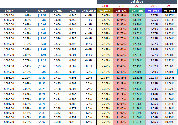
Keep in mind that the vol path is only for ATM vol. You can think of the ATM region of a smile sliding up and down a ramp of slope -1.0, -3.0, and so forth.

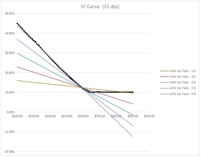
💡Notice that all of these ATM vol paths suggest a lower vol ATM vol at say the $675 strike than the actual smile implies. That is really a separate discussion, since skew is not really a “predictor” of vol anymore than a back-month future is a predictor of spot price. It is just a value that clears the market so it has risk-premiums embedded. It’s just another example of “real-world probabilities do not equal risk-neutral probabilities”. Even if that’s not satisfying, you could think of the skew as needing to average any number of price paths approaching a strike. If we drop $40 overnight, ATM IV is going to be higher than what the current $40 OTM put vol. If it takes 2 weeks, maybe not.

SPY skew is quite steep compared to most assets. A vol path that is tangent to the skew curve (-9.0 parameter) would be a very aggressive spot-vol correlation, especially considering that -1.0 is constant breakeven. Anything more negative means, as you rally, the value of an ATM straddle shrinks. That’s a strong clue that this slope idea is highly localized. If SPY doubles, the new ATM straddle isn’t going to be worth less than the current one, nevermind 0.

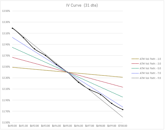
Zooming in on the strikes that are $5 around the ATM $695 strike:

How vol paths affect your delta

Once we’ve chosen a vol slope, we can compute the vol path, which in turn alters our model deltas. We can do this numerically, instead of deriving new formulas for greeks.

We are going to make a simplification, which is to assume that for a small spot move, changes in vol affect all the strikes by the same proportion. You are invited to think of what that would mean for implied skew. I plan to tackle that in a later article, but we’re building up in steps.

Let’s zoom in on the 695 call in the case when SPY goes up $1.

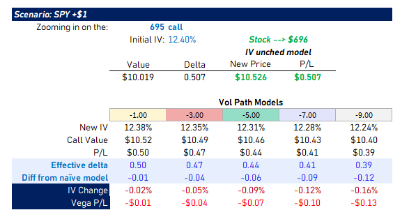
In the naive model, the 695 call goes up by its delta or $.507

But based on the different vol slopes, we know IV is going to fall from 12.4% to anything from 12.38% (-1.0 slope) to 12.24% (-9.0 slope). When we reprice the option with the lower vol, we see our profit is less than $.507. The difference, which is mechanically due to negative vega p/l, is being used to convey an “effective delta”.

If the market behaves as if the vol slope is -5.0, then instead of hedging the ATM call on a .507 delta, you should have used .44 delta.

[This is the topic I’m talking about at minute 37 in the context of estimating dealer hedging flows]

I show the vega p/l just to make the decomposition tie out between the recomputing of the option vs what it’s worth if IV was unchanged.

Vol beta

We’ll close by tying this dynamic back to hedge ratios in “delta one” vol products like VIX futures and ETPs.

VIX depends on a strip of options, not just ATM. But let’s stick with our simplification that IV changes proportionally across strikes such that if ATM vol decreases 10%, VIX falls 10% (not 10 percentage points but 10%…like 20 vol going to 18).

This is our IV projections according to different vol slopes for SPY shares up 1%:

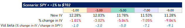
The vol slope parameter can be thought of as a vol beta. As in, what’s the beta of VXX shares to SPY?

[ I wrote about this last year during Liberation Day because on the sell-off, I bought both ES futures and VX futures but I needed to estimate the right ratio to buy them in.]

Running the regression for the past year in moontower.ai shows a VXX/SPY beta of -3.25:

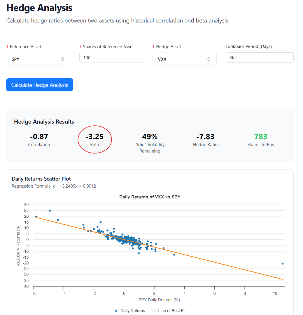
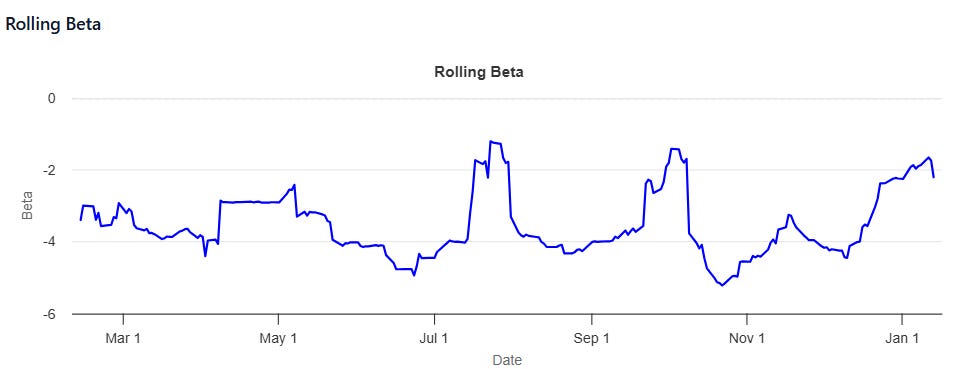
The rolling one-month beta is more volatile and would correspond to vol slopes between -1.5 to -5

Related video:

📺VXX Beta explained via Moontower Hedge Ratio Tool