Breakpoints

I caught David Boole’s segment about GME on CNBC because it was on Twitter. David used to cover me back when I showered every day. I agree with all of the framing.

He mentioned that the call skew in GME was higher this time around then back in early 2021. This made me want to look up the data but also prompted me to measure skew differently. But the “how to measure implied skew” question was a ball bouncing in my head already.

After publishing Scatterplot Gallery, Dave (not David Boole but an options market-maker) responded:

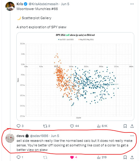
Dave is right. Sell side research likes normalized skew as a measure. So do I. We use it in moontower.ai. It’s how I looked at skew during my days at the fund and it’s the parameter I used at the spline points for my vol surfaces. I built up an intuition for those ratios over time per name. It’s also easy to compute.

Normalized skew is simple ratio of the volatility at an out-of-the-money point on the curve to the at-the-money volatility. It is common to measure at skew at the 25 and 10 delta strikes both on the upside and downside of the volatility surface and use the 50 delta option to normalize. (note the 50d strike is often but not always the at-the-money strike).

For example, assume:

Strike: 50 delta, IV: 28%

Strike: 25 delta put, IV: 32%

Normalized skew = OTM volatility/ ATM volatility - 1

Normalized skew = 32%/28% - 1 = 14.3%

The 25d put is trading at a 14% premium to the ATM volatility.

But…

Dave is CORRECT.

The measure doesn’t really make sense. It’s useful because it normalizes skew to ATM vol, but the measure often has a non-linear relationship itself to the vol. OTM options are sticky at the extremes of vol — so normalized skew flattens when vol gets high and steepens when it gets very low. So if you wanted to know if skew is “high” or “low” you still might want to condition it on vol level. Which of course, negates some of the benefit of normalizing it in the first place.

In general, it’s safe to use because it will correlate strongly with alternative measures of skew — it still captures “high” or “low”.

But unless you are a vol trader accustomed to how that parameter maps to prices because you see it in a model every day next to option premiums, it’s abstract.

Measuring surface and skew changes is a big topic in setting vol surfaces (or sheets if you’re “book a colonoscopy years old”).

Today, we’ll discuss skew models which will serve as background for next week’s paid post where we:

• look at another measure of skew in the spirit of Dave’s comment
• apply it to GME and David Boole’s comment

For both posts, we will be visual and lean towards simple.

Skew Models

Skew models allow traders to parameterize a vol surface. In other words, fit an IV curve to a discrete chain of strikes. From cubic splines to the vanna-vega-volga model, you can gorge yourself on as much complexity as you want.

Us knuckle-draggers who think an ecole is something you get from bad burger meat are just going to throw a line through some points. This is an example from the famous TT software:

The vol curve requires:

ATM or ATF VOLATILITY

Implying an ATM vol from the market or setting your own

BREAKPOINTS

Finding the IV of the strike at various moneyness, SD’s(standard deviation points) or deltas. Any of these measures is an attempt to measure the distance from the ATM strike to the “breakpoint” (ie 25 delta or 1 SD). Careful, moneyness is not a normalized measure. If a strike is 5% OTM, it’s much further away in a 10% vol name than a 50% vol name.

Example

The pictured model has 3 SD points above the ATM strike and below the ATM strike. Beyond 3 SD’s there will typically be a linear slope coefficient that fits the tails. That IV can then be parameterized by its ratio or spread to the ATM vol. So if the 25d put is 33% and the ATM put is 30% we are running a 25d put skew of 3 vol points or a ratio of 110%. As we’ll see, there’s no right way, just trade-offs.

Comments

• The goal is fit the market snugly but without creating arbitrages in the option premiums due to weird kinks. These curves interpolate vols for the strikes in between the breakpoints. Market makers play whack-a-mole with kinks that get out of line.
• Deal stocks or other assets with idiosyncratic behavior around specific price levels (think of how coal-switching puts a floor on nat gas prices) usually don’t have bell-shaped distributions. It’s hard to fit curves to them. Wrong tool for the job. That’s what Excel and some common sense is for.
• As mentioned earlier moontower.ai uses normalized skew by delta

On modeling skew changes

• “Sticky strike” refers to a model that assumes strike vols (vols at specific dollar strikes) stay fixed. This is reasonable over short horizons or smaller moves. It’s unlikely to hold over the time frame in which an OTM 30 strike put becomes far ITM
• “Sticky delta” means we expect IVs at various deltas to maintain a stable relationship with the ATM volatility. This is an implicit assumption if you use normalized skew — “I see that the 25d put seems to persistently trade at 110 to 115% of ATM vol”

There are hybrids and permutations. In a professional setting, that gamut ranges from highly bespoke proprietary models to a wide array of vendor software. I’ve used many types of models. Spot-vol correlation parameters were much more widely used in my second decade of trading. I’ve even used flat sheets, no skew at all. I’d just have a mental log of how far from flat sheets options of a particular distance from ATM would trade. I’ve used models that don’t have vols — everything is handled in price space. The models themselves were never a source of edge. But if a scale is consistently adding 2 pounds it’s still useful for comparison as long as you weigh everything with that scale.

This is why normalized skew is fine for cross-sectional comparison. It answers the question you're interested in even if it’s hard to interpret on its own. The truth is measuring skew is like trying to pinpoint a firefly from its sporadic bursts of light.

Consider a made-up $20 stock with a 6-month IV of 40%. I fit a dumb skew model to it (it’s an Easter egg for a certain group of people, all of whom likely have reading glasses by now).

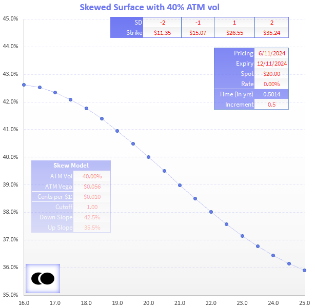
Things to notice:

1) Standard deviations are computed using 40% ATM vol. Those computations are explained in Using Log Returns And Volatility To Normalize Strike Distances.

2) Let’s look at the $24.50 strike. We can describe that strike in many ways:

• 22.5% OTM (moneyness breakpoint)
• .25 delta (delta relative breakpoint)
• .72 SD’s OTM (standard deviation breakpoint)

3) We can describe its skew:

• 3.9% clicks below ATM vol (spread relative)
• 9.8% discount to ATM vol (ratio relative aka normalized skew)

Like good little option taxonomists we can say lots of little things about our friend the $24.50 strike.

But now we shall kill him.

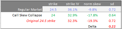
Some hedge fund wiseguy with an S&M fetish puts on a giant collar — buys puts and sells calls. Ravages the skew.

The ATM vol stays the same, the collar is vega-neutral. But we’ll assume the 24.50 call’s fixed strike vol drops from 36.1% to 32.3%, nearly 4 full clicks.

What can we say about this option?

• Well, it’s still 22.5% OTM.
• It’s still .72 standard deviations away since the ATM vol hasn’t changed (assume it happened quickly, so not much time elapsed).

The normalized skew has changed. The strike now trades at a 19.3% discount to the ATM vol (32.3/40 - 1).

That’s important. It tells us our measure is working — the call got hammered relative to the ATM and the discount got wider. Basic counting still works.

But we have a small problem.

If we parameterize our surface by delta we have a “nail Jell-O to the wall problem”. By virtue of the vol coming in, the delta at the strike also falls (this is also known as “vanna” — the Commander-in-Chief of greeks — getting both too much credit, blame, and airtime relative to its efforts).

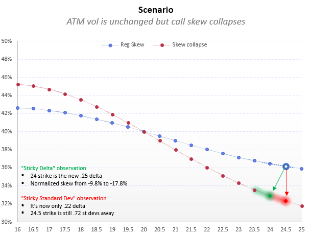
The $24 strike is now the .25 delta call. Its vol is 32.9%. If you are looking at skew changes using delta relative parameterization you will see skew fall from -9.8% to -17.8%. A steep drop but not quite the drop to -19.3% change if you used standard deviation relative or fixed strike relative breakpoints.

Summary:

Pictures are always better for these things:

The nuances of tracking skew changes are to finance what Equus Erotica is to sex. Like 40 people care.

Other sources

I’m not at liberty to blast it out but this was a widely-read piece on measuring skew:

You can also see Colin Bennett’s free book. My notes are here.

Just remember…

• The delta relative breakpoints are recursive in that the strike vols changing alters the strike deltas.
• SD relative breakpoints slide around with the ATM vol and time passing.
• Moneyness breakpoints jump around with every tick in the stock.

Whatever you pick, just be consistent and understand its biases. And when I say “you” I mean pros. If you are anyone else losing sleep over this, you’ve lost the script.

Options stuff is fun, “bicycle-for-the-mind” and all that. Just don’t think you need to know this. There’s no money printer at the end of this rainbow. It’s mostly useful for managing the risk of large option portfolios — the less stuff you trade the more irrelevant this stuff is.

You’ll go far in life if you can just be good enough to remember your hole cards and not need to check’em again to see if 3-7 offsuit is playable.