a sense of proportion around skew

Last week, we launched the Portfolio Visualizer in moontower.ai

It’s a tool for using vertical spreads to make directional bets.

Input: You enter a target price and expiration

Output: It shows you a matrix of every out-of-the-money strike combination up to the target in terms of what odds it pays.

A quick refresher on the utility of vertical spreads

I’ve written a lot about them but as a refresher, vertical spreads are clean ways to bet on a terminal price by a certain date.

• You know your max downside so you can put them on without worrying about being shaken out of them by marks. I call this “risk budgeting” a trade
• Spreads, especially tight ones, have largely offsetting greeks. When you use an outright option to bet on direction you are expressing a view on a basket of parameters in addition to direction — most notably volatility and its doppelganger time. You can be right on direction and wrong on the other parameters. Using options demands a view on volatility (ie the “volatility lens” I’m always droning about). Vertical spreads discard this requirement because the vol and time exposures are heavily neutralized.

The fussy reader will raise their hand, as they should.

“What about skew?

Doesn’t the implied skew impact the vol differential between the 2 strikes of a vertical spread?

How do I know if the odds are a good deal?”

These are awesome questions. Let’s get to work.

The goal: develop a sense of proportion about how much “high” or “low” skew impacts the odds

Payoff Visualizer

Let’s start with some odds.

We’ll look at the payoff odds for call spreads on SLV and USO etfs on trade date 2/25/2025.

We are looking at approximately .50d - .25d call spreads for expiry 4/17/2025.

In other words, buying roughly an ATM call vs selling a .25 delta call expiring in nearly 2 months.

SLV

Lower strike: $29.50

Lower strike implied vol: 24.9%

Higher strike: $32

Higher strike implied vol: 27%

Measured skew = .27 / .249 - 1 = +8.4% premium

The call spread is marked at $.57 vs a maximum value of $2.50 offering 3.4-1 odds if SLV expires above $32.

💡Note that if the 32 strike’s implied vol increased, all else equal, the spread would decline in value, the skew premium would be higher, and the buyer of the spread would get even better odds. It seems counter intuitive but by increasing the skew and pumping up the 32 strike call, the market is saying 2 things at once:

• the magnitude of the upside of the distribution is fatter (the call is expanding in value)
• the probability or hit rate of SLV going higher is lower — you are getting better odds to be long this binary outcome

This seemingly offsetting sentiment makes sense. If the upside magnitude is higher AND the hit rate is higher then the stock price must also be higher. But if we hold the stock price constant and just move the implied skew, then we are adding clay to the middle & downside of the distribution AND the further upside BUT removing it from the nearer upside.

In sum, silver has positive call skew and the .50d-.25d call spread with 2 months to expiry offers 3.4-1 odds.

Now let’s look at oil.

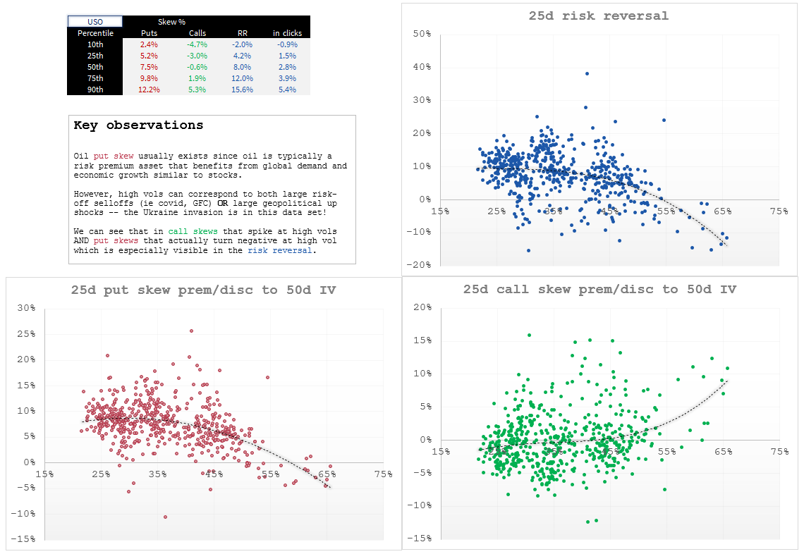
USO

Lower strike: $76

Lower strike implied vol: 27.9%

Higher strike: $81

Higher strike implied vol: 26.9%

Measured skew = .26.9 / .279 - 1 = -3.6% discount

The call spread is marked at $1.59 vs a maximum value of $5.00 offering 2.1-1 odds if USO expires above $81.

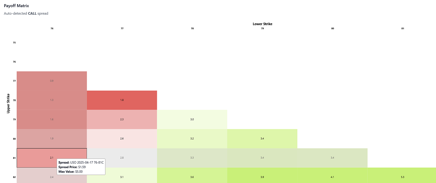
🔬What you should notice

USO vols are similar to SLV but the call spread .50d-.25 delta call spread is much more expensive (and pays less than 2/3 the odds of the SLV call spread). Skew is driving the disparity. In USO’s case, you are selling the topside call at discounted IV to ATM, but in SLV you selling a premium IV.

Weighing in on whether this is a structural mispricing of the probabilities is not where this post is going. That’s more of a research question. Knock yourself out, if you want to dig up the empirical distribution of returns. I can point to reasons why the skews look like this.

1) Spot-vol correlation

SLV vols tend to increase as silver rallies. Part of the precious metals as risk-off, fiat hedge rubric. Oil is a risk-on asset usually with demand for energy correlated with global demand growth. Like stocks, it has a negative spot/vol correlation. However in times of middle east geopolitical stress the spot/vol correlation can flip to positive.

2) Hedging

Producer hedging in oil markets tends usually involves buying puts or put spreads and selling calls. While consumers (ie airlines and refineries) are natural buyers of oil, their hedging requirements are typically swamped by producers.

[The vol inclined reader will notice that these reasons explain the skew but don’t rule out the call spreads being mispriced. The implied skew reflects the supply/demand for vol at various moneyness, but that’s not the same as saying the implied skew predicts the distribution. If you want to bet simply on directionality in a given time frame, taking advantage of the skew is a perfect use case for the risk-budgeted vertical spread. If you are not dynamically hedging, you are not concerned about the conditional behavior of vol as spot moves around.]

The key lesson of the discussion so far:

The level of skew, the percent premium/discount, is a major driver of the vertical spread price and therefore the payoff odds and implied probability.

An inferred lesson, that is not really surprising, is that different assets have different skews. Nobody is ever going to price a SPY surface with silver skews. Both the distributions and spot/vol correlations have different properties.

To develop a sense of proportion around how the range of measured skew affects payoff odds requires looking at assets idiosyncratic skew behavior. In moontower.ai, we display both time series for skew parameters as well as percentiles

Between knowing if the skew is “high” or “low” compared to history and seeing the payoffs in the visualizer we come to a practical questions that tie it altogether:

If .25d puts are in the 10th percentile vs the 90th percentile, how much is that going to change the odds offered on my put spread hedge?

If skew is at “average” levels what kind of odds should I expect on a 2-month .50-.25d call or put spread?

The remainder of the post will dive into these questions so you can walk away not only with a sense of proportion but be able to form your own rules of thumb so you can quickly handicap values like how much extra your paying for a put spread when skew is “low” or how much more your getting for selling a call spread when the OTM calls are cheap?

Here’s a few thoughts for everyone before we get to the paywall:

1) Tradeoffs

For a directional bet, I don't really see which spread to buy as a question of “what’s optimal?” You’d need an very fine-grained view of the distribution to identify that. Instead, I see a menu of tradeoffs between hit rate and payoff which the matrix displays naturally. In fact, just looking at the screenshots above of the matrix is very educational.

The matrix is the view I’d construct ad-hoc when I want to take a shot. I didn’t map the whole thing but I’d I basically run the same payoff calculation in my head by eyeballing a bunch of strikes, perhaps according to which option markets were tightest or have meaningful OI for liquidity purposes. It makes life easier to just have it organized in a matrix this way.

2) The hips and the fist

In any fighting sport you learn that power comes from the hips. The fist is just conduit that channels the power. When thinking about a directional bet, the work really is upstream of the options. The options are just the fist. It’s the easiest part. Most of the alpha power comes from the directional analysis. Or sticking your finger in the air.

Developing a sense of proportion about skew

We need to do 2 things to answer the practical question of how much does “low” or “high” skew in name change the value of the vertical spreads in real-life:

1. We need to see how much skew varies in a name
2. We need to run extreme skew parameters thru an option pricer to see how the spread’s price range (and therefore payoff odds) varies with the skew parameter’s range

Skew Variation

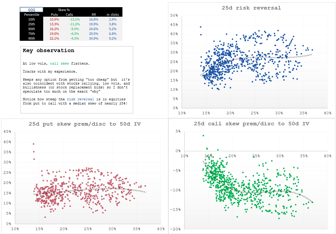
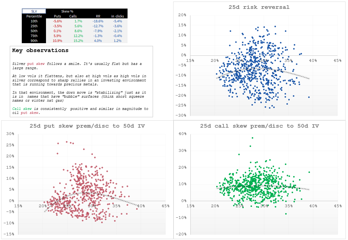
I did a small study of 3 names with different skew properties. I looked at 3 years of data to find the .50d IV as well as the .25d put and call skew parameters for options with about 2 months until expiry.

🗒️Notes on method

a) I allowed a tolerance of 50-70 days until expiry (that means there wasn’t necessarily a qualifying expiry for each trade date but there’s enough data points to get the gist).

b) Skew parameter = .25d IV / .50d IV - 1 … you can interpret that as a percent premium or discount to the .50d IV.

If .50d IV is 30% and the .25d put is 33%, then skew = +10%

💡Sometimes you’ll hear the term “clicks” or “vol points”. In this example, a 10% premium corresponds to 3 vol points or clicks.

Let’s just jump to the data which I think is mostly self explanatory now that you know the definitions. For each name I show the scatterplot of skew vs .50d vol level for:

a) .25d put

b) .25d call

c) .25d put - .25d call risk reversal

Remember unless it says “clicks” the skew parameter is in percent of .50d IV

USO

QQQ

SLV

Substack’s not the greatest for delivering these charts but you can always right click on the image and “open in new tab”.

The charts are nice because you can see that skew can vary with vol level. That’s discussed in the “key observation” stickies. Those stickies also show how skew is not some abstract idea — its specific behavior matches the specific properties of the underlying asset. Sometimes oil panics up or down. The tech index doesn’t panic up (even if single stocks in the index might).

We can get lost in reflecting when our goal was to see how much the skew varies in a name. This table will make it clear:

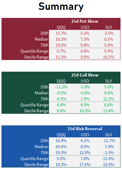
We can ignore the risk reversal. I included it because it took no extra effort. Instead, let’s focus on .25 skew. Again, just eyeballing, we can see that the interquartile ranges for put and call skews are typically around 5% wide (silver is a bit wider). Meaning that from the median to the 75th or 25th percentile you are only talking about changing the OTM option’s IV by about 2 or 3% of the .50d vol.

So if median put skew in QQQ is 16.2% premium to .50d IV and skew blows out to the 75th percentile than it goes to 19% premium.

If QQQ ATM vol is 20% your talking about a put IV going from 23.2% to 23.8%

How if QQQ IV is in the 25th percentile?

If ATM vol is 20% then the put is 13.3% premium or 22.7%

If skew went from the 25th percentile to the 75th, the put vol increases from 22.7% vol or 23.8% or just over 1 click.

Is one click a lot?

That’s the question we’re after.

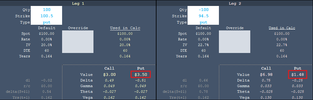
Put spread sensitivity

We can test this using a Black-Scholes calculator.

We can compute a 60 day .50d put at 20% IV vs a .25d put at 22.7% IV.

This represents “cheap” put skew in the 25th percentile.

We will do this on a hypothetical $100 stock.

The .50d put will be actually be in-the-money slightly as opposed to at-the-money.

[See Lessons from the .50 Delta option for an explanation]

We end up with the 100.50 strike vs the 94.50 strike. This $6 wide put spread represent the .25d wide put spread.

When the skew is “cheap”, the IV differential between the strikes is 2.7 vol points (ie 22.7% - 20%).

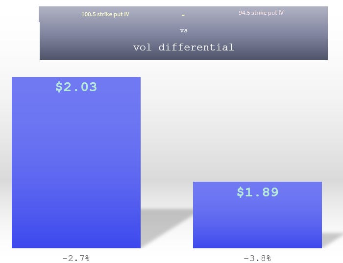
The put spread is worth $2.03

[The 100.50 put is worth $3.50 and the 94.5 put is worth $1.48]

If we raise the skew to the 75th percentile, the 94.5 put goes to 23.8% IV and a price of $1.62

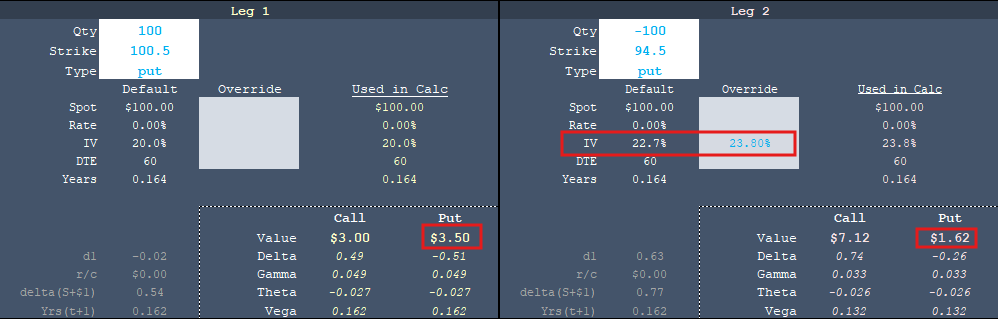
The put spread drops in value to $1.89

Again, notice when the put skew expands, the put spread drops in value! The left tail is getting fatter but the intermediate down move is losing distributional mass.

This is the put spread as a function of the vol differential between the 2 strikes. As the differential widens (the smaller put increasing relative to the .50d put) the spread gets cheaper.

What happens in odds space?

If the put spread is $2.03 and can be worth as much as $6.00 a buyer is getting 1.96-1 odds.

When the put spread gets cheaper, the buyer gets better odds of 2.17-1

In probability space, you go from 33.8% to 31.5% probability of expiring lower by expiry.*

The put spread changed in value by about $.15 on a $2 put spread as skew went from the 25th to 75th percentile all else equal. Given the variation of skew in QQQ it’s like every 3 cents in the put spread is 10 percentile points.

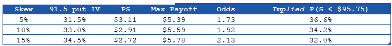
I won’t step thru it as slowly as I did with QQQ but here’s oil put spreads varying from 5% to 10% to 15% skew for the 100-91.5 put spread (.25d wide put spread):

Context is everything

When I was trading oil, a giant move in skew would mean, on a delta-neutral basis, a $5 wide spread would move 3 cents. If you made a nickel wide market on a put spread you’d be accused of making a market the broker could “drive a truck through”. In percentile space, you can see why.

But then again, you could argue that the exchange fees and broker commission represented a few percentile points.

If you are an options market maker, translating what low or high means to actual prices is important. It gives your market width context with respect to the surface parameters that you track. It lets you estimate how much edge you need to pad your market compared to how wrong you can be about how the surface might reprice.

On the other hand, if you are a purely directional trader the the difference in skew being low or high might be immaterial to your decision to take the odds unless your are able to discern probabilities down to just a few percent.

Now when you see a skew time series for a fixed maturity you know you can put the parameters in an option model and see just how much it changes the spread value.

You can derive your own sense of proportion customized to the context you trade in.

I’ll wrap by emphasizing that I’m writing from the perspective of mapping skew parameters to actual spread pricing. Trading skew on a delta-neutral basis because you think realized or implied vol will out or underperform as spot price travels across various strikes is a different animal. That is less about distributional outcomes and more about dynamic vol behavior. You care about what IV does when your vegas expand and contract, and what realized does as spot moves through your dollar gamma profile. It’s highly path-dependent. The opposite of a terminal risk-budgeted bet. In fact, the 2 different approaches can prescribe opposite trades meaning the risk-budgeted trader and the dynamic hedger can happily trade with each other. A classic example is the 1x2 ratio spread. The directional trader might use jacked put skew to buy a 1x2 put spread creating a highly attractive payoff profile in most scenario, while a dynamic hedger might be happy to own the 2 options because they expect vol to scream higher as the stock goes down.

For fun: What the most you’d be willing to pay for a $15/$10 1x2 put spread? The least? If you paid zero for it, can you lose?