crossing the commodity chasm

I was planning to publish a follow-up to last week’s derivative “income” bumhunting where I look closer at various ETF performances. I started data-wrangling and then got distracted with yesterday’s trade idea. I will circle back to the ETFs in an upcoming issue.

As far as the trade idea this is what I ended up doing:

• Liquidated most of my railroad shares (economic activity play that has held up well in contrast to commods)
• Shorted .54 delta calls in November expiry options in WTI. I used Z24 NYMEX crude options which are “Dec” options but expire in November. The nomenclature comes from the commodity delivery window as opposed to the last trading day of the options. Confusing if you are coming from equity land.
• Bought Dec2025 WTI futures

On balance, I added overrall risk-on length via the total quantity of Dec25 futures.

The oil legs assumed a .50 beta between Z25 and Z24 so I bought 2x as much Z25 as I sold in Z24 oil delta, which brings me to…commodity analytics. Like where did I get .50 beta from?

For some background, I spent 2005-2021 managing commodity options businesses. Despite moontower.ai being equity focused and the start of my career being in equities, ETFs, and equity options, commodity futures and options are my binkie.

One of my favorite periods of my professional career was building out the analytics for commodities. It was also a clue that I enjoyed building as much as trading. The career is most rewarding when you can not only drive the racecar but drive the one you built.

The analytics were similar to moontower.ai in the sense that they are volatility-centric and ignore fundamental data. But there is a tremendous amount of translation required to think about vol and term structure in the commodity markets.

A non-exhaustive list of features (or bugs) in commodity futures:

• Physical delivery and cash delivery nuances
• A single order book instead of multiple exchanges
• A large, opaque OTC market whose contracts are cleared by exchanges but not traded on them
• No insider trading rules
• Different rebate mechanisms for volume traders
• Less restrictions on market makers taking a “show” in voice markets
• Even the underlying is highly levered — and exchanges can change margin requirements on a whim
• Cross margining of look-alike products (ICE vs NYMEX WTI)
• Options on spreads, Asian options, “new crop”, short-dated ag options, and 0DTE has existed in these markets for almost 20 years already (but were not traded electronically)
• Close to 24 hour trading
• Early exercise of calls and puts in a world without dividends or corporate actions
• CFTC not SEC
• Different arbitrage bounds — a time spread can trade for a credit because each option expiry is tied to its own underlying. This gets very hairy in commodities that are hard to store (ie nat gas or electricity) or highly seasonal ones such as ags which have “new crop”/”old" crop” dynamics that can actually have negative correlations (the performance of an old crop will affect planting decisions for the next season — high prices one year can lead to oversupply the next. Forward vols in commodity markets are a fun topic.

Infrastructure-wise you need a totally different “security master” or database mapping between financial instruments.

• Underlyings can be referenced by many types of options in various combinations. Crack spreads, crush spreads, spark spreads. Options on all of them.
• Every commodity has different expiration schedules, trading hours, last trading time, settlement procedures, naming conventions.
• The markets pool liquidity in bespoke ways — October options in cotton are listed but never traded. If you trade nat gas you care a lot about 2 spreads in particular — H/J (March/April) and V/F (Oct/Jan). In RBOB, the gasoline spec for delivery changes in the North American summer.

Your security master needs to be flexible enough to accommodate all this variation. Your front-end analytics are going in the other direction — tuned for the idiosyncrasies of the markets you’re focused on. And then all the risk needs to be reported to central command in a way that fits with the overall portfolio risk while not losing the details when they matter. It is essential for the risk management layer to understand the drivers in these markets to devise appropriate shock scenarios and aggregations.

My first home in commodity trading was the oil complex. WTI, Brent, heating oil and gasoline (RBOB but I started trading it when HU was listed in parallel as the market was migrating to the RBOB spec). In that world you have American-style options expiries spanning from 1 day to many years into the future. You have calendar spread options (CSOs), crack options (I stood next to an independent trader that was long so many gas crack calls when Katrina hit that it was a noble percentage of a day’s worth of refining capacity in the US), Asian options, and European look-alike options that settled to swaps.

There were active markets in American vs European “switches”. You could exercise an American option for an hour after the market officially closed while the Europeans were cash-settled. If you were long Europeans on a strike, and short the Americans going into a pin…well, the market was gonna help you discover what that switch is worth.

If you trade WTI-Brent “arb” options, you are trading options on the spread between the 2 oil benchmarks. WTI and Brent have their own supply/demand dynamics because they are in different locations and vary by spec. This means different buyers and suppliers. Refineries optimize their throughput based on what end products are demanded and where (diesel, gasoline, jet fuel, bunker oil, etc). Throw in transportation costs, technicalities, and legality/tariff/sanctions on exports and you have a pair of highly liquid individual markets only loosely tethered by the wire of “arbitrage”. The arb options are a way to directly trade the spread. And then nerds can then relative value trade the vanilla options on each commodity vs the arb options. There’s no boxed arbitrage embedded in the math but the concept of implied pairwise correlation is a tradeable, albeit, messy parameter. And with the different expiration dates and times for the “same” month you will find yourself long or short a pile of unmatched option greeks for a string of days in between expirations (which also suggests that getting your volatility calendar correct is paramount).

(This implied correlation idea also exists in the context of calendar spread options. In 2007/2008 there were giant discounts in the WTI option forwards. The time spreads were incredibly attractive. The risk was you were inherently short spread vol so if you believed that the spread vol was highest conditional on the front month futures collapsing, then CSO puts were a clever hedge. The trade set-up was caused by the SEM Group blowout. I feel like I owe their desk a thank you for effectively buying my first apartment for me.)

An aside

The natural gas futures and options world is (was?) the king of cruft. It felt like a racket for churning exchange fees and broker commissions.

Expirations were so cumbersome because the liquid underlying was a physical future but the options that referenced them barely traded — instead the cash-settled options were traded but the cash-settled underlying swaps were not. They weren’t even listed, they were only cleared by the exchange! I can still remember being worried that I’d have an error, outtrade, or unreconciled position contaminate the grid I used to project how many futures I needed to buy/sell above/below each strike to replace the cash-settled deltas that were “going away”.

Oh yeah, and the swaps themselves had a different expiry than the futures so there were highly active markets in TAS (“trade at settlement”) futures, pen/LD swaps (“penultimate mini vs last day” swap spread), “futures/pen” (physical futures vs full penultimate swap), and the EFS (“exchange for swap” — last day futures vs last day swap). All of these things are tied together by algebraic relationships so you can triangulate the implied market in one from the legs of the others. Except none of this trades on a screen so you were still doing mock trading math based on quotes you are seeing on AOL IM or YM…in the 2010s!

I don’t remember the full history of how the markets eased into these conventions but I believe it was the marriage of disjointed OTC, exchange-traded, and physical markets. I’m not even getting into how the multipliers on these contracts work — if you trade X mmBTUs in the physical market that’s a size per # of days in the month which is how pipeline operators think and to which the financial players need to adapt.

And just like the oil market, there’s a NYMEX version and ICE version and sometimes you didn’t find out what you got until after the deal was consummated.

Hence venting on my Lost Xtranormal Video (Fonz, remember when we scripted this?)

It remains true that the number of commodities you can trade is much smaller than the number of equities, but there are loads of futures expirations, futures option expirations, strikes, and instruments.

A basic infrastructure starts with the futures chain and term structure. While I don’t currently have a proper infra I did grab several years of simple end-of-day WTI futures prices prompted by my oil trade idea.

I got distracted from writing the ETF post into creating a bunch of charts that demonstrate things I like to look at in futures. I’ll share them below and the reason a vol trader should care.

A quick comment on infrastructures.

You should be able to examine futures data in at least 2 ways:

1. Fixed expiration (ie a history of the Dec24 contract)
   
   This is especially useful for seasonal charts (ie X-axis is Jan thru Dec and the lines are contracts for various years)
   
2. Relative expiration (ie M1 or CL1)
   
   The ordinal number 1 refers to the first contract listed. This is the basis for “continuous” contracts. It’s also important because of the Samuelson effect which I mention in the interview with Dean — a contract with 12 months until expiry is less volatile than the same contract with 1 month until expiry. Which is another way of saying the M1-M12 spread has volatility and that volatility has its own properties.

The importance of having both views compounds when we layer in option analysis.

We’ll keep to a tight format. A chart and its relevance. All data is WTI futures settlement on the NYMEX.

[LLM note: To organize the data there was one instance where I wasn’t sure the easiest way to do it in Excel. I figured I’d need a helper column but instead of trial-and-error I just gave ChatGPT a screenshot of the spreadsheet and a description of my desired output. Abracadabra. Even the explanation for how the formula worked was perfect. I don’t know how long until it’s here but I feel like sometime shortly, organizing the data, laying out the charts, and the blog post will all be done by autonomous parallel AI agents. Come to think of it, why would I even prompt it…the LLM will just prompt better questions than I’m bothering to answer just by knowing what data is in front of me and the history of my blog posts.

The movie Fight Club makes more sense to me now than it ever did before.

Nerds being the victim of their own success is the own goal the Colosseum has been waiting for]

Alright, let’s get to it.

We start with a couple high level charts. They are useful when inspecting a commodity for the first time to get a sense of its nature.

Term structure time series chart

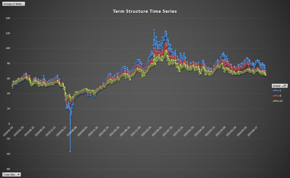
• To keep it legible, I just chose 3 ordinal months — M1, M8, M15. You can see how steep the contango was in April 2020 when the front month went negative!
• You can also see how for the past 5 years, the oil price has been backwardated (descending term structure) whenever the prompt price has been at least $45. I didn’t load the data from the 2010s but the last few years have been regime. Perhaps reflecting the idea that oil-demand in the future is uncertain with the focus on alternative fuels. (Personally I keep my core oil length in the deferred futures incentivized by an implied positive roll return and because the mandate also comes with a lowered incentive to invest in supply. In other words, vibes. I don’t know anything about the future but energy is part of my asset allocation. Hedgers sell the back so that’s where there should be a compensation for providing liquidity which manifests in a roll return. If I have to pick a spot on the curve to fill that bucket, that’s where I’m going.)

Term structure cloud chart

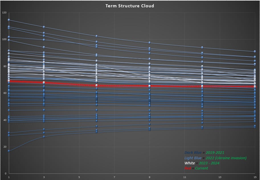
• I group term structures by month and average them. Looks like a vol cone doesn’t it.
• The back end has a tighter range than the front. It’s less volatile. Supply and demand are more elastic with a year to go than with a month to go.

Volatility term structure is one of the most important tradable concepts for option traders. Time spreads, straddle swaps, implied forward vols. So here’s the kind of riddle I might give in an interview:

There’s 3 contracts listed — M1, M2, M3

They each have their own option chains and the ATM implied vols are 30% across the board.

1) Is the option term structure flat, ascending, or descending?

2) Give me a framework for computing the forward vol.

Instead of an answer, I’ll offer a clue:

The vol ratio cloud

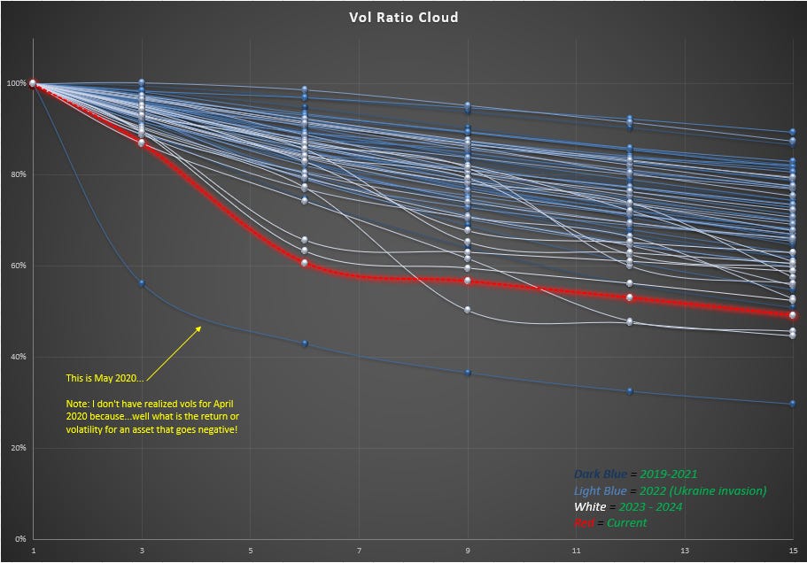
• This is a chart of 1 month realized volatility for each contract divided by M1’s realized volatility (grouped by month)
• Notice how some periods of time the back months are far less volatile than the near months. I think of this as volatility in the futures spread absorbing the volatility from the back months as the near month is being driven by some current concern that is not propagating to the backs. May 2020 being the archetypical example as we were running out of near term storage during COVID.
• How does this idea inform your thinking about the riddle above?

Zooming in on spread volatility

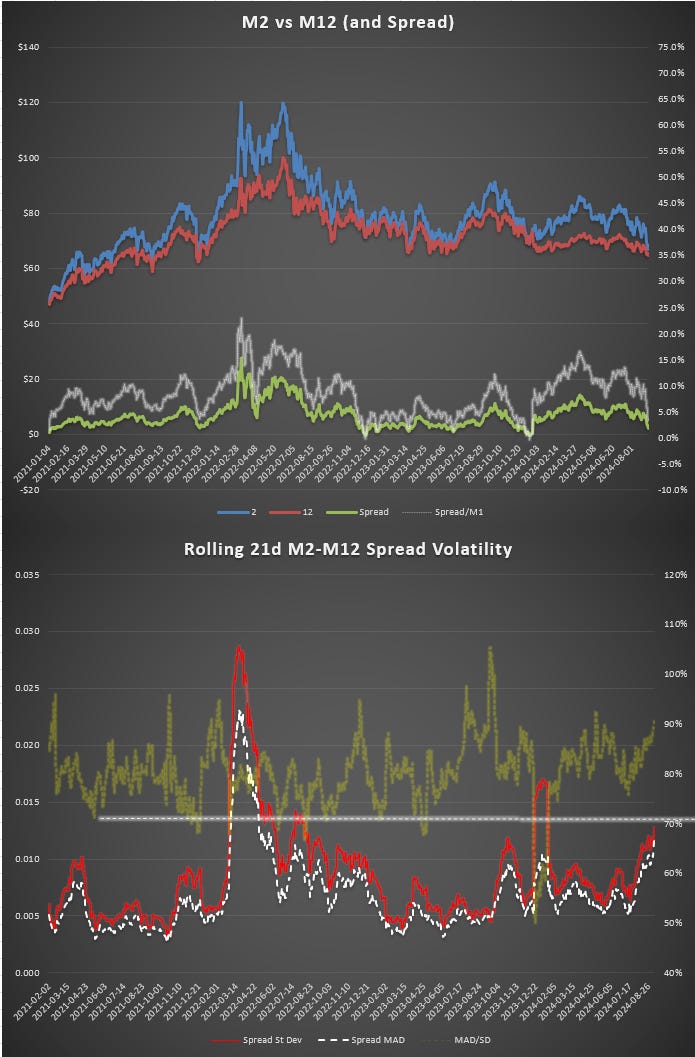
To reduce the noise from M1 a tad we focus on the M2/M12 futures behavior from Jan2021 until last week.

In the top panel we see:

• Time series of both futures prices. This is not a continuous roll return display so at each expiry as M2 inherits M3’s price there’s a small bump in futures prices that you would adjust for if you were working in a returns context.
• The green time series of the futures spread defined as M2 - M12 (front - back is a commodity convention but the equity market defines it the opposite way. Another source of confusion and “Texas” hedging for traders who cross the chasm from commods to equities or vice versa). Notice that the spread has been positive (a backwardated market) for almost the entire period.
• The silver time series just normalizes the spread value by the M2 price into percent terms.

In the bottom panel:

• The red line is the rolling 21d standard deviation of the spread price changes. The spike is the Ukraine invasion where the near-dated futures skyrocketed relative to the backs. Inelastic demand in the front meets supply concerns. We don’t compute percent volatility (what if a spread price is zero or negative) but instead measure the price volatility directly.
• The white line is the MAD or “mean absolute deviation”. This measure of volatility tends to be lower since we don’t amplify large moves by squaring them as we do with standard deviation.
• The army green line (right axis) is the MAD/St Dev ratio. An MAD less than .80 typically signifies a skewed or fat-tailed distribution of moves. See the [👿MAD Straddle for more color on this idea.]

Spread “delta”

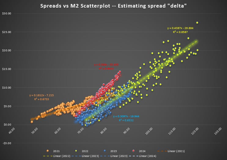
This is a scatterplot of spread price vs M2 price.

The slope of the regression tells us the “spread delta”. For example in 2022 (yellow), a $1 change in M2, meant a $.44 change in the spread.

If you are long the futures spread (long M2 and short M12), you are inherently long the market. If you want to isolate your trade to just betting on the slope between the 2 prices you must weight the position by the spread delta. So for each M12 you sell, you buy only .44 M2.

This comes in handy if you are trading a large options book with deltas in each month. You normalize them all to M1 deltas as a quick, liquid hedge. The r2 of the regressions give you a sense of how volatile that delta estimate is. A lower r2, a worse fit. If the fit is relatively poor, you will likely delta hedge your spreads directly and more often to reduce the noise.

A few observations:

• 2021 & 2022: the underlying had a wide range of M2 prices
• 2021 and 2023 had the lowest r2 indicating more variation in the spread “delta”
• Spread delta is highest in 2024 ($.57 change per $1 move in M2)

This observation brings us to the last chart. A high spread delta typically means a wider divergence between contracts as M2 moves around. The spread is volatile. If the front month goes up a dollar, the back month “lags” more than if the spread delta were lower.

Say it however you like:

• More volatile spreads mean that the volatility ratio between the back and front is lower.
• The beta is lower.
• The back is not “keeping” up with the front.

We can observe this directly by looking at each of those years’ M12/M2 realized vol ratio.

Notice that the high spread delta of 2024 corresponds to a low M12/M2 vol ratio.

In 2021, when the spread delta is a mere .18, the vol ratio between the 2 months spends plenty of time above 80% and even goes above 100% as the futures curve moved in parallel rather than flattening/steepening.

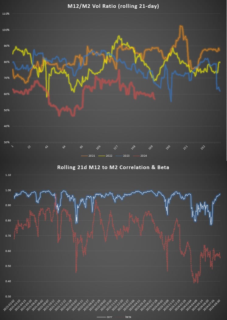
Can you see how spread volatility and vol ratio would have profound influence on how to interpret the options term structure on these contracts?

If the spread volatility is high, meaning the realized vol ratio of M12 to M2 is low, then if you are long time spreads you are going to be short options on the thing that moving a lot, and long options on the thing that’s lagging. You want to make sure you are getting the appropriate vol discount to hold that! Measuring what that is will get you to a proper understanding of the vol term structure and implied forward vol.

If you are coming from equity vol land, where the options are struck on the same underlying this is a new frontier for you.

We close with the bottom panel which simply shows the rolling correlation and beta (beta is vol ratio * correlation). This is the correct number to use for weighting your future positions not just the aforementioned vol ratio. The beta can change due to the vol ratio or the correlation and it’s worth decomposing it to see what’s driving the inevitable mismatch between your hedge ratios and realized p/l.

Trading commodity vol after trading equity vol can feel like a foreign world at first. But trading equity vol from trading delta one is an even bigger leap. Once you get used to commodities they actually feel cleaner. I’m super rusty on thinking about early exercise, dividends, rev/cons, and merger-arbish math because all those muscles atrophied from a life in commods.

Even the strange commodity trades I talk about with Dean in the interview revolve around USO and UNG — commodity trades that got tangled with SEC wrappers.

Commodities have their own language and their own grammar. But they are globally pertinent and tell their own gripping stories of history. I’ve recommended it before, but Javier Blas and Jack Farchy’s book World For Sale is an absolute banger. The best book I’ve read in my last 20.

Let’s leave it there.